Quantum I

Compilation of notes for Quantum I class for Spring 2023.

The Basics

The Basics

The Wavefunction
- Written in 1 spatial dimension as $\Psi (x,t)$.
  - Can be complex
  - Will suppress the inputs from now on, unless needed
- It’s evolution is given by the Time Dependent Schrodinger equation
  - $i \hbar \frac{\partial \Psi}{\partial t} = \frac{-\hbar^{2}}{2m}\frac{\partial^{2} \Psi}{\partial^{2} x}+V\Psi$
Born’s Statistical Interpretation:
- The probability of finding the particle between a and b is given by
 - $\frac{\int_{a}^{b} |\Psi|^{2}dx}{\int_{-\infty}^{\infty} |\Psi|^{2}dx}$
 - Denominator is typically 1 because functions we care about are typically normalized
- Classically: Assume there is some $P(x,t)$ that gives the probability of a particle appearing at x at time t
 - $ <x(t)> = \int_{\infty}^{\infty} xP(x,t)dx$
 - $\int_{-\infty}^{\infty} P(x,t) dx = 1$
 - Suppose we have some operator Q. The expectation value:
 - $ <Q(t)> = \int_{\infty}^{\infty} QP(x,t)dx$
- Quantum: We are given a wave function $\Psi(x,t)$. You then get:
 - $ <x(t)> = \int_{\infty}^{\infty} x|\Psi|^{2}dx$
 - $\int_{-\infty}^{\infty} |\Psi|^{2} dx = 1$
 - Suppose we have some operator Q. The expectation value:
 - $ <Q(t)> = \int_{\infty}^{\infty} \Psi^{*}Q\Psi dx$
Velocity/momentum
$<x(t)> = \int_{\infty}^{\infty}x|\Psi|^{2}dx$
$v = \frac{d}{dt}<x(t)> = \int_{\infty}^{\infty}x \frac{\partial}{\partial t}|\Psi|^{2}dx$
- $\frac{\partial}{\partial t}|\Psi|^{2} = \Psi^{*}\frac{\partial \Psi}{\partial t}+\Psi\frac{\partial \Psi^{*}}{\partial t}$
- From Schrodinger’s equation, can replace:
 - $\frac{\partial \Psi}{\partial t} = \frac{i\hbar}{2m}\frac{\partial^{2}}{\partial x^{2}}\Psi-\frac{i}{\hbar}V\Psi$
- Taking the conjugate of Schrodinger’s equation (assuming V is real):
 - $\frac{\partial \Psi^{*}}{\partial t} = \frac{i\hbar}{2m}\frac{\partial^{2}}{\partial x^{2}}\Psi^{*}-\frac{i}{\hbar}V\Psi^{*}$
- Subbing into above yields:
 - $\frac{\partial}{\partial t}|\Psi|^{2} = i\frac{\hbar}{2m}(\Psi^{*}\frac{\partial^{2} \Psi}{\partial x^{2}} - \Psi\frac{\partial^{2}}{\partial x^{2}}\Psi_{*}) = \frac{\partial}{\partial x}(\frac{i\hbar}{2m}(\Psi^{*}\frac{\partial \Psi}{\partial x}-\Psi\frac{\partial \Psi^{*}}{\partial x}))$
- Hence:
 - $\frac{d}{dt}<x(t)> = \int x\frac{\partial}{\partial x} (\frac{i\hbar}{2m}(\Psi^{*} \frac{\partial \Psi}{\partial x} - \Psi \frac{\partial \Psi^{*}}{\partial x}))$
- Integrate by parts , and utilize the boundary conditions that $|\Psi(x)|^{2} \rightarrow 0$ and $|\Psi^{*}(x)|^{2} \rightarrow 0$ at $\pm \infty$
 - $v = \frac{d}{dt}<x> = \int \Psi^{*} (\frac{-i\hbar}{m} \frac{\partial}{\partial x}) \Psi$
- We call operator $\hat{p} = -i\hbar \frac{\partial}{\partial x}$

The Current Density Operator (probability current)

probability current J is defined as $\hat{J}(x,t) = \frac{i\hbar}{2m}(\Psi\frac{\partial \Psi^{*}}{\partial x}-\Psi^{*}\frac{\partial \Psi}{\partial x})$
We can think of this as the “flow” of probability across a boundary
Can be derived by finding $\frac{\partial}{\partial t}|\Psi|^{2}$
- rewrite this time derivative using Schrodinger’s equation
- Use conservation of probability: $\frac{\partial}{\partial t}|\Psi|^{2} = -\frac{\partial J}{\partial x}$
Rationale: Imagine a wavefunction as a plane wave:
- $\Psi(x,t)=Ae^{i(kx-\omega t)}$
- $P=|\Psi|^{2}=|A|^{2}$
- $J = \frac{\hbar k}{m} |A|^{2}$
  - $\frac{\hbar k}{m}$ has units of speed, and $|A|^{2}$ is a probability density, so J can be interpreted as a probability flux

Erenhfest’s Principle

P1:
- $<v> = \frac{d}{dt}<x>$
- Namely, that quantum mechanic predictions approach the classical predictions
P2:
- The equivalent of Newton’s Law in Quantum Mechanics
- $\frac{d}{dt} = -<\frac{\partial V}{\partial x}>$
 - Write out the formula for the expectation value of $p = -i\hbar\frac{\partial}{\partial x}$
 - Expand out derivatives and utilize equivalence of mixed partials to swap $\frac{\partial^{2}}{\partial t \partial x}$ to $\frac{\partial^{2}}{\partial x \partial t}$
 - Use Schrodinger’s equation to substitute first order time derivatives with second order spatial derivatives (Don’t forgot to conjugate for $\Psi^{*}$ term!)
 - Use integration by parts twice in a row to eliminate $\frac{\partial^{3}}{\partial x^{3}}$ term (remember the boundary conditions $\Psi(\pm \infty) \rightarrow 0$ and $\Psi^{*}(\pm \infty) \rightarrow 0$)
 - Expand all the partials and things should cancel to P2 of Erenhfest’s Theorem

Uncertainty Princple

$\sigma_{i} = \sqrt{<i^{2}>-^2}$
for a coordinate and its associated momentum:
- $\sigma_{x}\sigma_{p_{x}} \geq \frac{\hbar}{2}$
For a coordinate with another coordinate:
- $\sigma_{x}\sigma_{y} \geq 0$
For a momentum with a momentum:
- $\sigma_{p_{x}}\sigma_{p_{y}} \geq 0$
For a coordinate with a momentum that isn’t it’s own:
- $\sigma_{x}\sigma_{p_y} \geq 0$

Time Independent SE

$\Psi(x,t) = \psi(x)\phi(t)$ is only possible iff $V(x,t) = V(x)$
Making this assumption, use seperation of variables, take the partials. You will notice that the LHS only depends on time and the RHS only depends on space. So each side must equal some constant (call this constant E)
- The time equation yields $\phi(t) = \phi(0)exp(\frac{-i Et}{\hbar})$
  - $\omega=\frac{E}{\hbar}$ as shorthand
  - $\phi(0)$ is a constant at $t=0$
- The space equation (called the Time Dependent Schrodinger Equation) is:
  - $\frac{-\hbar}{2m}\frac{d^{2}\psi}{dx^{2}}+V(x)\psi(x) = E\psi(x)$
    - Alternatively: $\hat{H}\psi = E\psi$
    - This is an eigenvalue problem in an infinite dimensional space
- So $\Psi(x,t) = \psi(x)exp(\frac{-iEt}{\hbar})$
- Observe that $|\Psi(x,t)|^{2}$ is independent of time
- the expectation value of any time-independent operator is time-independent
- Importantly, the expectation value of the energy is independent of time and has a definite value ($\sigma_{E} = 0$).
  - Corresponds to the Hamiltonian $\hat{H} = \frac{-\hbar^2}{2m}\frac{\partial^2}{\partial x^2} + V(x)$
- Also, all other expectation values of operators are time independent

Interference of Stationary States

Suppose that we are dealing with the time-independent Schrodinger Equation. The general time evolution of the wavefunction in a stationary potential is:
- $\Psi(x,t)=\Sigma_{n=1}^{\infty}c_{n}\psi_{n}(x)exp(\frac{-iE_{n}t}{\hbar})$
  - $\Sigma|c_{n}|^{2}=1$
  - If we want to Fourier decompose a function $f(x)$ in terms of the eigenfunctions $\Psi_{n}$, we can write the $c_n$ as $c_{n} = \int \Psi_{n}(x)^{*} f(x) dx$
Suppose that you have the state:
- $\Psi(x,t)=c_{1}\psi_{1} exp(\frac{-iE_{1}t}{\hbar})+c_{2}\psi_{2} exp(\frac{-iE_{2}t}{\hbar})$
 - This implies (assuming that the stationary states are real eigenfunctions and you have real coefficients): $|\Psi(x,t)|^{2}=c_{1}^{2}\psi_{1}^{2}+c_{2}^{2}\psi_{2}^{2}+2c_{1}c_{2}\cos(\frac{(E_{1}-E_{2})t}{\hbar})$
- Looking at the expectation value of $\hat{Q}$, we get
 - $<Q> = |c_{1}|^{2}Q_{11}+|c_{2}|^{2}Q_{22}+ {c_{1}}^{*}c_{2}Q_{12} + {c_{2}}^{*}c_{1}Q_{21}$
 - $Q_{ij} =\int_{\infty}^{\infty}\psi_{i}^{*}\hat{Q}\psi_{2} dx$
 - called matrix elements

Solving TISE

Remember the boundary conditions:
- $\Psi(\pm\infty)\rightarrow 0$
- At each interface:
  - The wavefunction is continuous ($\psi_{l}=\psi_{r}$)
  - The derivative of the wavefunction is continuous (usually, there are some exceptions like the delta function) ($\frac{d\psi_{l}}{dx}=\frac{d\psi_{r}}{dx}$)
  - You can also use symmetry arguments if appropriate

$V(x)=V_{0}$

$E>V_{0}$
- $\frac{\partial^{2}\psi}{\partial x^{2}} = \frac{-2m}{\hbar}(E-V_{0})\psi(v)$
  - Let $k^{2}=\frac{2m}{\hbar}(E-V_{0})$
  - $\psi(x)=Ae^{ikx}+Be^{-ikx}=C\cos(kx)+D\sin(kx)=A\sin(kx+\delta)$
$E<V_{0}$
- Let $k^{2}=\frac{2m}{\hbar}(V_{0}-E)$
- $\frac{\partial^{2}\psi}{\partial x^{2}} = k^{2}\psi(v)$
 - $\psi(x)=Ae^{kx}+Be^{-kx}=C\cosh(kx)+D\sinh(kx)$
- Classically forbidden

Infinite Square Well

The well has a width of $a$
The walls of infinite height occur at $x=0$ and $x=a$
Energies: $E_{n}=\frac{\hbar^{2}n^{2}\pi^{2}}{2ma^{2}}$
Wavefunctions: $\psi_{n}=\sqrt{\frac{2}{a}}\sin(\frac{n\pi x}{a})$

Properties of Eigenfunctions

Symmetric potentials have symmetric eigenfunctions
All eigenfunctions are muthually orthogonal
- $\int \psi_{m}^{*} \psi_{n} = \delta_{mn}$
- For the infinite square well, useful orthogonality relations include:
  - $\int_{0}^{a} sin(\frac{n\pi x}{a})sin(\frac{m\pi x}{a}) = \frac{a}{2}\delta_{mn}$
  - $\int_{0}^{a} cos(\frac{n\pi x}{a})cos(\frac{m\pi x}{a}) = \frac{a}{2}\delta_{mn}$
  - $\int_{0}^{a} cos(\frac{n\pi x}{a})sin(\frac{m\pi x}{a}) = 0$
Any other function can be represented as a sum of the eigenfunctions (complete set of state)
- This means that you can write the time evolution of a wavefunction $f(x)$ as $\Psi(x,t) = \Sigma_{n=1}^{\infty}c_{n}\psi_{n}(x)exp(\frac{-iE_{n}t}{\hbar})$
- The coefficients can be found via $c_{n} = \int \psi^{*}_{n}(x)f(x)dx$
- Probability must be conserved though ($\Sigma_{n}c_{n}^{2}=1$)

Finite Square Well

$V(x) = -V_0$ between -a to a, and equals $0$ otherwise
$\psi(x) = Be^{kx}$ for $x \leq -a$, $\psi(x) = C\sin(lx)+D\cos(lx)$ for $-a \leq x \leq a$, and $\psi(x) = Fe^{-kx}$
Match the functions and derivatives at the boundary to yields
- $k = l\tan(la)$
  - $k=\sqrt{\frac{2m(E)}{\hbar^{2}}}$
  - $l = \sqrt{\frac{2m(E-V_{0})}{\hbar^{2}}}$
  - Solve for the value of E that solves this equation (transcendental)
    - To do this, the above can be rewritten in terms of $z=la$ and $z_0 = \frac{a}{\hbar}\sqrt{2mV_0}$, and then solve for z
    - $tan(z) = \sqrt{(\frac{z_0}{z})^2-1}$
    - For a wide and deep well ($z_0$ is big), we get an infinite square well with only the odd states and offset by $V_0$
    - For a shallow and narrow well, we approach the delta well
  - You can find the transmission coefficient $T = \frac{|F|^2}{|A|^2}$ and see that periodically, the well becomes transparent ($T=1$)

Dirac Delta Function

$V(x) = -\alpha\delta(x)$
- if $x=0 \rightarrow \delta = \infty$
- if $x\neq 0 \rightarrow \delta = 0$
- $\int_{-\infty}^{\infty}\delta(x)dx = 1$
- $\int_{0}^{-\infty}f(x)\delta(x-a)dx = f(a)$
On the LHS and RHS, you just get growing exponentials on the left and decaying exponentials on the right. Call the parameter $\kappa = \frac{\sqrt{2mE}}{\hbar}$
From the continuity of the wavefunction, we know the coefficients of the LHS and RHS match (call this coefficient B)
We can’t assume that the derivative is continuous. Taking a step back, let’s look at the TISE:
- $\frac{-\hbar}{2m}\frac{d^{2}\psi}{dx^{2}}+V(x)\psi(x) = E\psi(x)$
- Integrate w.r.t. x from $-\epsilon$ to $\epsilon$ (ie. in a small region around zero) to get
  - $\frac{-\hbar}{2m}(\frac{d\Psi_{L}}{dx}\rvert_{-\epsilon}-\frac{d\Psi_{R}}{dx}\rvert_{\epsilon})+\int_{-\epsilon}^{\epsilon}V(x)\psi(x) = \int_{-\epsilon}^{\epsilon}E\psi(x)$
    - $\Psi_{L}$ and $\Psi_{R}$ is the wavefunction on the left and the right
  - Let $\epsilon$ go to zero. The RHS goes to zero, and if V(0) is finite then the 2nd term on the LHS is zero. Hence $\Psi_{L}=\Psi_{R}$
  - If V(0) is infinite, then you need to take into account the value of the 2nd LHS term. This also means that $\Psi_{L}$ and $\Psi_{R}$ are NOT equal to each other.
- For the Dirac delta, we know what $\Psi_{L}$ and $\Psi_{R}$ and we know $\int_{-\epsilon}^{\epsilon}-\alpha\delta(x)\psi(x) = -\alpha B$
- Doing the algebra yields $\kappa = \frac{m\alpha}{\hbar^{2}}\rightarrow E = \frac{-m^{2}\alpha^{2}}{2\hbar^{2}}$
- So we only have a single bound state with energy $E = \frac{-m\alpha^{2}}{2\hbar^{2}}$ with eigenfunction $\Psi_{L}=\frac{\sqrt{m\alpha}}{\hbar}e^{-\frac{m\alpha|x|}{\hbar^2}}$
- The scattering states have any energy $E>0$
  - Both sides of the equation have sinusoidal solutions. Matching continuity of function, taking into account discontinuity of the first derivative, and assuming only incidence of particles from the left ($G=0$), we find that (with $\beta=\frac{m\alpha}{\hbar^2k}$)
    - $B = \frac{i\beta}{1-i\beta}A$
    - $F = \frac{1}{1-i\beta}A$
    - Transmission and reflection coefficients can be found from F and B respectively

Free Particle

$\frac{-\hbar^{2}}{2m}\frac{d\psi^{2}}{dx^{2}} = E\psi$
Solutions are $\Psi = Ae^{ikx}+Be^{-ikx}$ where $k = \frac{\sqrt{2mE}}{\hbar}$
We can add on the energy dependent phase to see that the two states represent right and left moving waves respectively
- Not normalizable
  - We can take sums of various k values to construct normalizable functions
  - Define a right moving wave:
  - $\Psi(x,t) = \frac{1}{\sqrt{2\pi}}\int_{=\infty}^{\infty} \phi(k)exp(i(kx-\frac{\hbar^{2}k^{2}}{2m}t))$
  - $\Psi(x,0) = \frac{1}{\sqrt{2\pi}}\int_{=\infty}^{\infty} \phi(k)exp(ikx)$

Fourier Transform Definition

Define the Fourier Transform as:
- $f(x) = \frac{1}{\sqrt{2\pi}}\int_{\infty}^{\infty}F(k)exp(ikx)$
- $F(k) = \frac{1}{\sqrt{2\pi}}\int_{\infty}^{\infty}f(x)exp(-ikx)$
If we make the correspondence: $f(x)\rightarrow \Psi(x,0)$ and $F(k) \rightarrow \phi(k)$, then we can calculate the Fourier components of any moving wave packets (ie. decompose any wave packet in terms of complex exponentials of various magnitude)
We also have the problem that the speed of the packet is twice the classical speed. This is because of the distinction between the group velocity ($v_{g} = \frac{d\omega}{dk}$) and the phase velocity ($v_{p} = \frac{\omega}{k}$)

Scattering States

Flux of a particle is $k|C|^{2}$, or in words, it is the momentum of the particle times the probability density
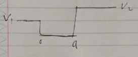
Define a potential such that $V(x) = V_{1}$ for $x<0$,$V(x) = 0$ for $0<x<a$,$V(x) = V_{2}$ for $x>a$
For scattering problems, $R = \frac{k|B|^{2}}{k|A|^{2}}$ and $T = \frac{k^{’}|F|^{2}}{k|A|^{2}}$
- To remember which k is assigned to each probability, look at the region where the wave exists in and choose this momentum
For a symmetric potential well, at widths of integer multiples of half wavelength, you get perfect transmittance

SHO

Define $[A,B] = AB-BA$ to be the commutator where A and B are operators
The SHO (simple harmonic oscillator) has the potential of the form $V(x) = \frac{(m\omega x)^{2}}{2m}$
- $\omega^2 = \frac{k}{m}$
The central idea of solving the harmonic oscillator via ladder operators is to rewrite the Hamiltonian $H = \frac{1}{2m}[p^{2}+(m\omega x)^{2}]$ in terms of ladder operators

Commutation relation of $\hat{x}$ and $\hat{p}$

$[\hat{x},\hat{p}] = i\hbar$
You utilize this ad nauseum for Angular momentum operators and, in this case, ladder operators

Ladder Operators

Let $a^{+} = \frac{1}{\sqrt{2\hbar\omega m}}(-i\hat{p}+m\omega\hat{x})$ be the creation/raising operator
Let $a = \frac{1}{\sqrt{2\hbar\omega m}}(i\hat{p}+m\omega\hat{x})$ be the annihilation/lowering operator
- Alternatively, this can go the other way around where you rewrite $\hat{x}$ and $\hat{p}$ in terms of the raising and lowering operators
  - $\hat{x} = \sqrt{\frac{\hbar}{2m\omega}}(a_{+}+a)$
  - $\hat{p} = i\sqrt{\frac{\hbar m \omega}{2}}(a_{+}-a)$
H can be rewritten as $H = \hbar\omega aa^{+}-\frac{\hbar\omega}{2} = \hbar\omega a^{+}a+\frac{\hbar\omega}{2} $
$[a,a^{+}] = 1$
Applying the Hamiltonian to $a^{+}\psi$ and utilizing the commutators shows that $H(a^{+}\psi) = (E+\hbar\omega)a^{+}\psi$
Analogously, we get that $H(a\psi) = (E-\hbar\omega)a\psi$
- There exists a ground state to the system since $V(x) = \frac{1}{2}m\omega^{2}x^{2} \geq 0$. In words, you can’t lower the energy to a negative value
- Let $a\psi_{0} = 0$, where $\psi_{0}$ refer to the ground state. Applying a to this eigenstate kills the wavefunction
  - Expand out what a is and solve the dif eq to get (after normalization)
    - $\psi_{0} = (\frac{m\omega}{\pi\hbar})^{\frac{1}{4}}exp(\frac{-m\omega x^{2}}{2\hbar})$
    - To get the ground state energy, apply H to $\psi_{0}$ to get $E_{0} = \frac{\hbar\omega}{2}$
We can recursively apply $a^{+}$ to $\psi_{0}$ to generate the higher quantum level eigenfuctions and eigenvalues: $\Psi_{n} = \frac{1}{\sqrt{n!}}(a_{+})^{n} \Psi_0$
Alternatively, the general eigenfunctions are $\psi_n(x) = (\frac{m\omega}{\pi\hbar})^\frac{1}{4}\frac{1}{\sqrt{2^n n!}}H_n(\xi)e^{\frac{-\xi^2}{2}}$ where $\xi = \sqrt{\frac{m\omega}{\hbar}}x$ where $H_n$ are the Hermite polynomials

Hermetian Operators

$<Q> = \int \phi^{*} \hat{Q} \phi dx = <\phi|Q\phi>$
- We define Hermetian operators such that $<f|\hat{Q}f> = <\hat{Q}f|f>$
 - All observables can be represented by hermetian operators.
 - The expectation value of hermetian operators is real
- The hermetian conjugate (or the adjoint) of an operator is denoted $Q^{\dagger}$ such that $<f|\hat{Q}g> = <\hat{Q^{\dagger}}f|g>$ for all f and g
- An operator is hermetian if $Q = Q^{\dagger}$
The eigenvalues and vectors of a hermetian Q satisfy $Q\psi = q\psi$
- All eigenvalues of hermetian operators are real
- All eigenfunctions of distinct eigenvalues of hermetian operators are orthogonal

Momentum Eigenvalues

Let $f_{p} = \frac{1}{\sqrt{2\phi \hbar}} e^{\frac{ipx}{\hbar}}$ be the eigenvector of the equation $-i\hbar \frac{d}{dx} f_p = p f_p$
- Satisfies the orthogonality relation $<f_{p’}|f_{p}> = \delta(p’-p)$
- Any function can then be written as $\frac{1}{\sqrt{2\pi\hbar}}\int_{-\infty}^{\infty} c(p) exp(\frac{ipx}{\hbar})$ where $c(p)$ is given by the Fourier trick
 - $c(p) = <f_{p’}|f>$

Fourier transforms

$\phi(p,t) = \frac{1}{\sqrt{2\pi\hbar}}\int_{-\infty}^{\infty} exp(\frac{-ipx}{\hbar}) \psi(x,t) dx$
$\psi(x,t) = \frac{1}{\sqrt{2\pi\hbar}}\int_{-\infty}^{\infty} exp(\frac{ipx}{\hbar}) \psi(p,t) dx$
$phi(p,t)$ is the wave function in the position basis, and holds equivalent information to the wavefunction in position basis
- $x = i\hbar \frac{\partial}{\partial p}$ is position basis

Generalized Uncertainty Relationship

Let A and be B be Hermitian operators. Then
- $\sigma_A^{2} \sigma_B^{2} \geq |\frac{<[A,B]>}{2i}|^{2}$
- This is derived using the definition of the variance $\sigma_A^2 = <A-<A>\Psi^{*}|A-<A>|\Psi >$
 - You then use the Schwartz Inequality $f^2g^2 \geq |<f|g>|^2$ where f and g are complex numbers, as well as the inequality that $|z|^2 \geq Im(z)^2$ where z is complex
To find a minimum uncertainty, we want both of the inequalities to the equalities. Doing this, we find that
- $g(x) = ia f(x)$ where $a$ is real
- In particular, if we let $g(x) = p-|\Psi>$ and $f(x) = x-<x>|\Psi>$, we get a differential equation of the form
 - $\frac{d\Psi}{\Psi} = \frac{-ax}{\hbar}++\frac{a<x>}{\hbar}+\frac{i}{\hbar} dx$, where the expectation values are constants. Solving this, we get that
 - $\Psi(x) = Aexp(\frac{-ax^2}{2\hbar}+\frac{a<x>x}{\hbar}+\frac{i}{\hbar}x) = A’ exp(\frac{-a(x-<x>)^{2}}{2\hbar})exp(\frac{ix}{\hbar})$
 - This is a Gaussian
Another important relation is $\Delta E\Delta t \geq \frac{\hbar}{2}$
- Look at $\frac{d}{dt}<Q> = <\frac{\partial \Phi}{\partial t}|Q\Phi>+<\Phi|\frac{dQ}{dt}\Phi>+<\Phi|Q\frac{\partial \Phi}{\partial t}>$
- From Schrodinger’s equation, we know that $\frac{\partial \Phi}{\partial t} = \frac{-i}{\hbar}H\Phi$. Plug this in above to get that
 - $\frac{d}{dt}<Q> = \frac{i}{\hbar}<[H,Q]>+<\frac{\partial Q}{\partial t}>$
- Combine the above with the Generalized Uncertainty Principle where A=H and B = Q, and define ($\frac{\sigma_Q}{\hbar<Q>} = \Delta t$), we can prove the energy time uncertainty

Dirac Notation

Have been using it throughout these notes
The only weird thing is the projection operator $\hat{P} = |a><a|$
- This operator picks out the portion of any other vector that lies along a
 - $P|b> = <a|b>|a>$
 - $\Sigma_{n}|e_{n}><e_{n}| = 1$ is the identity operator. Can be inserted into any dirac notation expression with whatever basis you want
 - Need to remember that $<p|x> = \frac{1}{\sqrt{2\pi\hbar}}exp(\frac{-ipx}{\hbar})$

Solution to Spherically Symmetric Schrodinger’s Equation

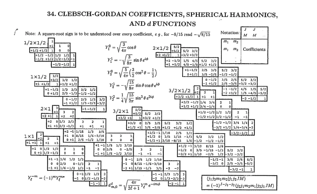
The angular solutions take the form of spherical harmonics:
- $Y_{l}^{m}(\theta,\phi) = \sqrt{\frac{(2l+1)(l-m)!}{4\pi (l+m)!}}e^{im\phi}P^m_l(\cos\theta)$
  - $P_{l}(\cos\theta)$ are the associated Legendre polynomials
  - These are orthonormal functions
The radial equation becomes
- $\frac{-\hbar^2}{2m}\frac{d^2 u}{dr^2}+(V+\frac{\hbar^2}{2m}\frac{l(l+1)}{r^2})u = Eu$
  - $u(r) = rR(r)$
- For a general hydronic atom
  - $E_{n} = -(\frac{\mu}{2\hbar^2}(\frac{(Ze^2)}{4\pi \epsilon_{0}})^2)\frac{1}{n^2}$
  - We also define the Bohr Radius as $a = \frac{4\pi \epsilon_{0}\hbar^2}{\mu Ze^2}$
  - The final normalized wavefunctions are $\Phi_{nlm} = \sqrt{(\frac{2}{na})^3\frac{(n-l-1)!}{2n(n+l)!}}e^{-\frac{r}{na}}(\frac{2r}{na})^{l}L^{2l+1}_{n-l-1}(\frac{2r}{na})Y_l^m(\theta,\phi)$
    - $L_q(x) = \frac{e^x}{q!}(\frac{d}{dx})^q(e^{-x}x^q)$

Angular Momentum

NOTE: A general rule of commutators: $[AB,C] =A[B,C]+[A,C]B$
$[L_x,L_y] = i\hbar L_z$
- Cyclic permutations hold (x->y->z)
- Anticommutative
$L^{2}$ commutes with $L_{x}$,$L_{y}$ and $L_{z}$
- This means that $L^2$ can have simultaneous eigenstates with a direction. Let’s take $L_{z}$ to be said direction
  - $L^2f = \lambda f$ and $L_{z}f = \mu f$
  - Define the ladder operators $L_{\pm} = L_{x}\pm L_{y}$
  - $[L_{z},L_{\pm}] =\pm \hbar L_{\pm}$
  - $[L^2,L_{\pm}] =0$
- This means that $L_{\pm}f$ is also an eigenfunction of $L_{z}$ with a new eigenvalue $\mu \pm \hbar$.
- Let $L_{z}f = \hbar l f$ where l is an integer
- $L^{2} = L_{\pm}L_{\mp}+L_z^2\mp \hbar L_{z}$
$L_{\pm}|lm> = \hbar \sqrt{l(l+1)-m(m\pm 1)}|s(m\pm 1)>$
$L^{2}|lm> = \hbar l(l+1)|lm>$
$L_{z}|lm> = m\hbar |lm>$
$l$ can take either half or integer values

Spherical Coordinates

$L_{x} = -i\hbar (-\sin\phi \frac{\partial}{\partial \theta}-\cos\phi\cot\theta \frac{\partial}{\partial \phi})$
$L_{y} = -i\hbar(\cos\phi\frac{\partial}{\partial \theta}-\sin\phi\cot\theta\frac{\partial}{\partial \phi})$
$L_{z} = -i\hbar \frac{\partial}{\partial \phi}$
$L^{2} = -\hbar^2[\frac{1}{\sin\theta}\frac{\partial}{\partial \theta}(\sin \theta \frac{\partial}{\partial \theta})+\frac{1}{\sin^{2}\theta}\frac{\partial^2}{\partial \phi^2}]$
The only reason you would ever use these forms is to calculate the explicit eigenfunctions of these operators

Spin

Has the same commutator relationships as angular momentum
In matrix form, for spin 1/2, we have
- $S^{2} = \frac{3}{4} \hbar^2 \begin{pmatrix} 1 & 0\\ 0 & 1 \end{pmatrix}$
- $S_{+} = \hbar \begin{pmatrix} 0& 1\\0&0 \end{pmatrix}$
- $S_{-} = \hbar \begin{pmatrix} 0& 0\\1&0 \end{pmatrix}$
- $S = \frac{\hbar}{2} \sigma$
  - $\sigma_{x} = \begin{pmatrix} 0 & 1\\1&0 \end{pmatrix}$
  - $\sigma_{y} = \begin{pmatrix} 0 & -i\\i&0 \end{pmatrix}$
  - $\sigma_{z} = \begin{pmatrix} 1 & 0\\0&-1 \end{pmatrix}$

Electron in Magnetic Field

The magnetic moment is defined as $\mu = \gamma S$ where $\gamma$ is the gyromagnetic ratio
The Hamiltonian of the system becomes $-\mu\cdot B = -\gamma B\cdot S$
- Suppose that we have a B field configured like $B = B_{0} \hat{k}$. For an electron, we have 2 possible energies whose eigenfunctions are the same as $S_{z}$
- Writing down the time evolution of the system and taking the expectation value of $S_{x}$, $S_{y}$ and $S_{z}$, we find that the spin vector makes an angle of $\alpha$ to the z axis and precesses around the z-axis with frequency $\omega = \gamma B$

Addition of Angular Momenta

Suppose that you have two particles in states $|s_{1}m_{1}>$ and $|s_{2}m_{2}>$ where the notation $|sm>$ denotes a particle of spin s with quantum humber m
Denote the composite states as $|s_{1}s_{2}m_{1}m_{2}>$, or alternatively as $|s_{1}m_{1}>|s_{2}m_{2}>$
- The new z quantum number is just $m = m_{1}+m_{2}$
- The new total spin is kind of indeterminate. By this, I mean that the composite particle has the potential to have a variety of total spins (ie. a superposition of total spins)
  - For instance, combining two spin 1/2 particles could yield either a spin 0 particle or a spin 1 particle
  - In general, given a spin $s_{1}$ and a spin $s_{2}$ particle, the possible total spins range from $s_{1}+s_{2}$ all the way down to $|s_{2}-s_{1}|$
Let’s look at combining two spin 1/2 particles. Start with the composite state $|\frac{1}{2}\frac{1}{2} m_{1}m_{2}>$. You can repeatedly apply the normalized raising and lowering operators $S^{\pm}$ on the state with the highest possible spin (ie. 1)
- Once You exhaust all the possible spin 1, move onto spin 0
- You get the following for spin 1 (triplet):
  - $|11> = |\frac{1}{2}\frac{1}{2}\frac{1}{2}\frac{1}{2}>$
  - $|10> = \frac{1}{\sqrt{2}}(|\frac{1}{2}\frac{1}{2}\frac{1}{2}\frac{-1}{2}>+|\frac{1}{2}\frac{1}{2}\frac{-1}{2}\frac{1}{2}>)$
  - $|1-1> = |\frac{1}{2}\frac{1}{2}\frac{-1}{2}\frac{-1}{2}>$
- And the following form spin 0 (singlet):
  - $|00> = \frac{1}{\sqrt{2}}(|\frac{1}{2}\frac{1}{2}\frac{1}{2}\frac{-1}{2}>-|\frac{1}{2}\frac{1}{2}\frac{-1}{2}\frac{1}{2}>)$
In general, you can state that
- $|sm> \Sigma_{m_1+m_2=m} C_{m_1 m_2 m}^{s_1 s_2 s} |s_1 s_2 m_1 m_2>$
- And conversely $|s_{1}s_{2}m_{1}m_{2}> = \Sigma_{s} C_{m_1 m_2 m}^{s_1 s_2 s} |sm>$ for ($m = m_1 +m_2$)
- The constants are called the Clebsch-Gordan coefficients and they are a fancy look up table
  - NOTE: Take the square root of the absolute value in the cell, then apply the negative sign as needed

The Basics#

The Current Density Operator (probability current)#

Erenhfest’s Principle#

Uncertainty Princple#

Time Independent SE#

Interference of Stationary States#

Solving TISE#

$V(x)=V_{0}$#

Infinite Square Well#

Properties of Eigenfunctions#

Finite Square Well#

Dirac Delta Function#

Free Particle#

Fourier Transform Definition#

Scattering States#

SHO#

Commutation relation of $\hat{x}$ and $\hat{p}$#

Ladder Operators#

Hermetian Operators#

Momentum Eigenvalues#

Fourier transforms#

Generalized Uncertainty Relationship#

Dirac Notation#

Solution to Spherically Symmetric Schrodinger’s Equation#

Angular Momentum#

Spherical Coordinates#

Spin#

Electron in Magnetic Field#

Addition of Angular Momenta#

The Basics

The Current Density Operator (probability current)

Erenhfest’s Principle

Uncertainty Princple

Time Independent SE

Interference of Stationary States

Solving TISE

$V(x)=V_{0}$

Infinite Square Well

Properties of Eigenfunctions

Finite Square Well

Dirac Delta Function

Free Particle

Fourier Transform Definition

Scattering States

SHO

Commutation relation of $\hat{x}$ and $\hat{p}$

Ladder Operators

Hermetian Operators

Momentum Eigenvalues

Fourier transforms

Generalized Uncertainty Relationship

Dirac Notation

Solution to Spherically Symmetric Schrodinger’s Equation

Angular Momentum

Spherical Coordinates

Spin

Electron in Magnetic Field

Addition of Angular Momenta