Imagine that you have a 1D chain. You have two species in the chain at each lattice site.
Define the Hamilton to be $H = \Sigma_{i} (t+\delta t) C_{Ai}^{\dag} C_{Bi} + (t-\delta t) C_{A(i+1)} C_{Bi}^{\dag}$
Think of C as fermion creation and annihilation operators at a particular lattice site
If $t = \delta t$, then there are only interactions between A and B molecules in a local pair
If $t = -\delta t$, now you couple B at site i with A at site i+1
Imagine that the distance between each lattice site can be written as $a$
We can decompose the operators into a Fourier basis
$C_{Ai} = \Sigma_{k} exp(ika_{i}) C_{Ak}$
$C_{Bi} = \Sigma_{k} exp(ika_{i}) C_{Bk}$
After some massaging (break into sub matrices), we can write the model as $H = \Sigma_{k} \begin{pmatrix} C_{Ak}^{\dag} C_{Bk}^{\dag} \end{pmatrix} (H(k)) \begin{pmatrix} C_{Ak} \\ C_{Bk} \end{pmatrix}$
$H(k) = d_{j}(k) \cdot \sigma_{j}$
$\sigma_{j}$ are the Pauli matrices
The d functions are some scalar functions, which can be bundled into some vector
$d_{x} = (t+\delta t)+ (t-\delta t) \cos(ka)$
$d_{y} = (t-\delta t) \sin (ka)$
$d_{z} = 0$
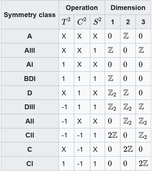
This is a C=0, T=0, S=1 model
Plotting the d vector, we see that there are two cases:
$\delta t> 0$: Traces a circle which crosses the positive x-axis twice
$\delta t<0$: Traces a circle which circles the origin
This vector encodes the winding number (0 and 1 for $\delta t >0$ and $\delta t <0$ respectively)
If you diagonalize H(k), we see that there is no difference in the spectrum between the possible $\delta t$ values
Explicitly, we see that $\epsilon_{k} = \pm | \vec{d}(k)|$, which follows from diagonalizing a Hamilonian of the form $H = \Sigma_{i} a_{i} \sigma_{i}$
Let’s generalize a bit:
Suppose that we have a 1D chain which maintains the sublattice symmetry (ie. there is hopping between sublattices, but not within a sublattice), we get a Hamiltonian in an analagous form to the SSH model, but we have a H(k) of the form $ \begin{pmatrix} 0 & h_{k} \\ h_{k}^{\dag} & 0 \end{pmatrix}$
The winding number then becomes: $\nu = \frac{1}{2\pi i} \int dk \frac{\partial}{\partial k} (\log (\det h(k)))$
$ka \in (-\pi, \pi)$
This integral can be done via complex contour integration with $z = exp(-ika)$ as the integration variable
This is restricted to integers (can be positive, negative, or zero)
Let’s jump to the 2D case. Assume only a sub-lattice symmetry. You maintain the off block diagonal structure of the fourier modes, but now your Hamiltonian can be a function of two wavenumbers ($H(k_{x},k_{y}) = \vec{d}(k) \cdot \sigma$)
In order to maintain the sub-lattice symmetry, we need to allow $d_{z}$ to be non-zero
Convert the $\vec{d}$ to spherical coordinates
For concreteness, choose a system which fixes the length of $\vec{d}$. You can plot $\vec{d}$ on the surface of a sphere
Suppose that $\theta_{k}=0$. Observe that there is an ambiguity in what $|->_{k}$ (can be multiple values at the south pole)
You can try to fix this by adding an arbitrary phase to your wavefunctions, but then the north pole is ill-defined
Hence, you might need multiple gauge choices in different regions in order to have well-defined wavefunctions across the entire Hilbert space
When you do this, you need to be very careful that your gauge choices smoothly transition between each region
Related to this idea is the so called the Berry Connection: $\vec{A_{k}} = -i <u_{k} | \vec{\partial_{k}} u_{k}>$ where u is your wavefunction
This is dependent on your gauge choice: $\tilde{A}(k) = A_{n}(k)+ \nabla_{k}\beta(k) $ where $\beta$ is your gauge transformation
The Berry phase is then defined as the closed path integral: $\gamma = \int_{C} d\vec{k} \cdot A_{n}(k) $
This is the phase difference that you pick up from moving a state very slowly around the curve
We can use Stokes theorem to rewrite the Berry phase in terms of a surface integral: $\gamma_{n} = \int dS \cdot \Omega_{n}(k)$
$\Omega_{n}(k) = \nabla_{k} \times A_{n}(k)$ in 3 dimensions is the Berry curvature
In exact analogy to in E&M where the vector potential has some gauge transformation and you need to calculate the field strength tensor to get observables like the EM fields
We know that the above integral must equal an integer multiple of $2\pi$, where the multiple is the so called Chern number
If we have two regions covering out space, then they must agree with each other on the boundary up to some phase. Integrating this phase difference over the length of the boundary gives a $2\pi$ integer multiple as per the above argument (any accumulated phase difference from gauge differences obeys Chern’s theorem)
The winding number for this system is then $\frac{1}{2\pi i} \oint dz \frac{\rho’(z)}{\rho(z)}$
Only the j zeros of $\rho(z)$ contribute (ie $\rho(z_{j})=0$)
What is the mode associated with some $z_{j}$ zero of the system?
Find some $\phi$ such that $H\phi = 0$
Make the ansatz $\phi = \begin{pmatrix} \Sigma_{n=1}^{\infty} z_{j}^{n-1} |n> \\ 0 \end{pmatrix}$ where $z_{j}$ is the zero of the
You find that you have $H \phi = \begin{pmatrix} 0 \\ \hat{Z} \Sigma_{n=1}^{\infty} z_{j}^{n-1} |n> \end{pmatrix}$. You can expand $\hat{Z}$ in terms of the translation operators and do some relabelling of the indices to see that the bottom term is 0 due to $\rho(z_{i}) = 0$
Remember Bloch’s theorem:
Assume that $H = \frac{\vec{p^{2}}}{2m}+ V(\vec{r})$ with the discrete symmetry $V(\vec{r}+\vec{a}) = V(\vec{r})$ for your lattice spacing
NOTE: not assuming rotational symmetry, just using the shorthand $\vec{r} = (x,y)$
The wavefunction then must obey $\phi_{n\vec{q}}(\vec{r}) = \phi_{n\vec{q}}(\vec{r}+\vec{a}) = exp(i\vec{q}\cdot\vec{a}) \phi_{n\vec{q}} (\vec{r})$ where $\vec{q} = \frac{2\sigma{\vec{n}}}{L}$ is the quasi-momentum (L is the length of our box which arises from imposing periodic boundary conditions on our system)
Apply some electric field in the y direction. This can be accomplished by perturbing the momentum: $\vec{p} \rightarrow \vec{p}+ \frac{e}{c}\vec{A}(x)$ where $\vec{E} = -\frac{1}{c} \frac{\partial \vec{A}}{\partial x}$
Apply a unitary transformation: $H \rightarrow exp(-i\vec{q}\cdot \vec{r}) H exp(i\vec{q}\cdot \vec{r})$ and $\phi \rightarrow exp(-i\vec{q}\cdot \vec{r})\phi$ yields the Hamiltonian: $H_{q} = \frac{(\vec{q}+\vec{p})^{2}}{2m} + V(\vec{r})$ (ie. the momentum gets shifted)