Following the book “Understanding Digital Signal Processing” by Richard G. Lyons.
Discrete Sequences and Systems
Definitions and Notation
- Signal Processing: the science of analyzing time-varying physical processes
- Analog refers to waveforms that are continuous in time and can take on a continuous range o amplitude values
- Comes from analog computers, where physical electronic differentiators and integrators were used to model differential equations
- Discrete: the time variable is quantized
- This means that the signal at intermediate values is unknown. You can make pretty good guesses at intermediate values, but ultimately, you don’t know
- A discrete system is one which takes in some input stream(s) $x_{i}(n)$ and returns some output streams $y_{j}(n)$ where n denotes which discrete time step you’re dealing with
- A fundamental difference of discrete systems from analog systems is the sampling rate $f_{s}$, which is typically independent of the signal you’re sampling
- An alternative representation of any discrete signal is in the frequency basis via Fourier transforms. Hence, $x(n) \rightarrow X(m)$ where m indexes the frequency (m=0 is the DC component)
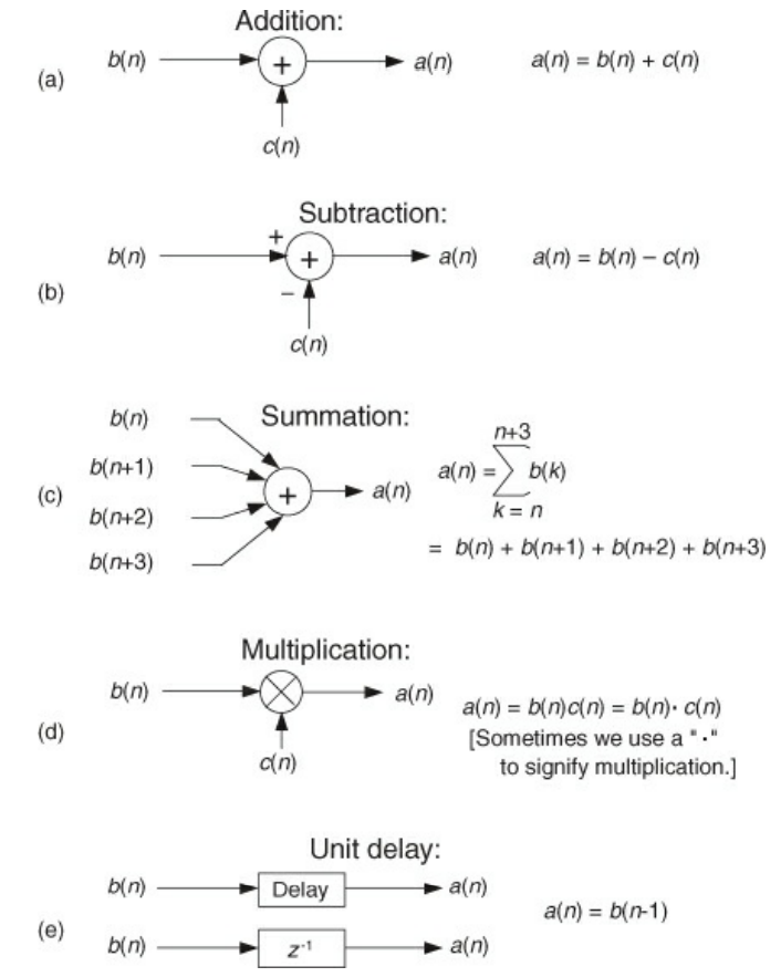
- Basic signal processing operation symbols
Decibel
- Fun history lesson: The original power difference was in units of “bels”, where the power difference is $10 * log_{10}(\frac{P_{1}}{P_{2}})$ bels
- This was inconvenient, since you routinely measured power differences smaller than that. so the decibel was introduced to account for this (just multiply by 10!)
- The log scale lets us compare signals of wildly different orders of magnitude on the same plot
Linear and Time-Invariant Systems
- A linear System obeys the homogeneity property: $c_{1} x_{1}(n)+c_{2} x_{2}(n) \rightarrow c_{1} y_{1}(n)+c_{2} y_{2}(n) $
- This system is also commutative
- A time-invariant system is one where a time delay/shift in the input sequence causes an equivalent time delay in the output sequence. To wit: $x(n+k) \rightarrow y(n+k)$
- Given a time-invariant linear system (LTI), we can determine the output response via a convolution of the input sequence with system response to a unit impulse signal (ie. a signal where $x(0) = 1$ and all other times are 0)
- The frequency response of a LTI system via a discrete Fourier transform of the impulse response
Periodic Sampling
Frequency Ambiguity
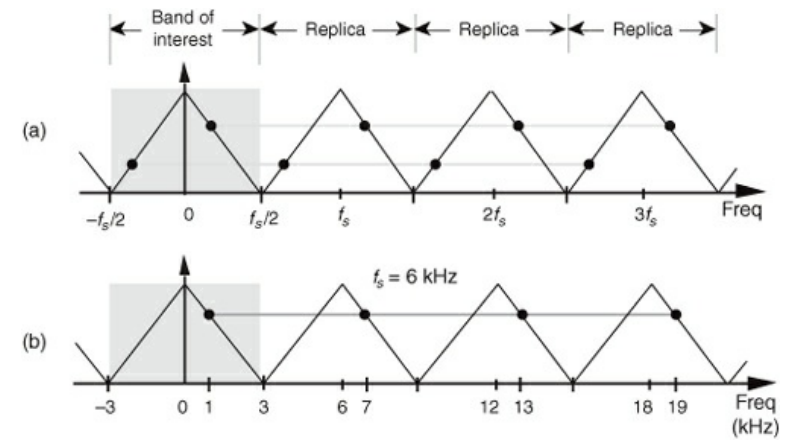
- When sampling at a rate of $f_{s}$ samples/second, if k is an integer, you can’t distinguish sampled values of a sinewave of $f_{0}$ Hz and a sinewave of $f_{0}+kf_{s}$ Hz
- Suppose that you have a Shark’s tooth frequency response
- The region of interest is based around 0, with a spread of $f_{s}$
- Outside this region in both directions, the band of interest gets repeated
- Because of this copying, any signal you measure in the band of interest cannot be differentiated by an equivalent signal in some other band
- This arises due to convolution
Low Pass Aliasing
- This frequency ambiguity shows up when dealing with low pass signals (ie. the spectral energy is all below some cutoff frequency B)
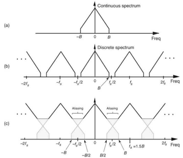
- The above demonstrates the problem
- graph A represents the continuous incoming signal
- graph B represents the sampled spectra when the sampling rate is $f_{s} \geq 2B$ (so called Nyquist criterion). All of the frequency bands are nicely separated from each other
- graph C represents the sampled spectra when the sampling rate is less than the Nyquist criterion. As you can see, you get crossing of bands, which corrupts the initial signal
- You won’t know the amplitude in the cross over regions a priori
- All of the frequency content outside of the band gets folded into it when sampling (regardless of Nyquist criterion) (see above)
- This necessitates analog low pass filtering prior to sampling
BandPass Filtering
- Sometimes, we care more about the bandwidth of a signal (ie. the range of frequencies that we can measure) compared to the absolute frequency that we can measure
- As such, we want to be able to sample some range of frequencies around some non-zero $f_{c}$ such that the result is centered around 0
Band Pass Aliasing
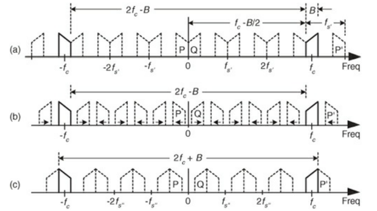
- The above shows how aliasing can be a problem with band pass signals
- We want to downshift the band by $f_{c}-\frac{B}{2}$ at some sampling frequency $f_{s}$. This means that we need to close a distance of $2f_{c}-B$ between the upper edge of the negative frequencies and the lower edge of the positive frequencies
- Because of the spectral replication, we can fit $m*f_{s}$ in this gap, where m is some positive integer
- Hence: $m*f_{s} = 2f_{c}-B$ or $f_{s} = \frac{2f_{c}-B}{m}$
- Increasing the frequency past this point for fixed m will shift the P band right and the Q band left, causing aliasing. Hence, $\frac{2f_{c}-B}{m}$ gives an upper bound on $f_{s}$
- What happens if you decrease $f_{s}$? In Fig. b, the P lobe gets shifted down, and the Q lobe gets shifted up. Hence, there is some lower bound where the bands start to overlap again.
- This occurs when the lower edge of the negative frequencies and the upper edge of the positive frequencies match. This distance is $2f_{s}+B$
- Because you’re shifting the other way, you need to add one more band in the mix. Hence, the lower bound is $f_{s} = \frac{2f_{c}+B}{m+1}$
- Hence we have: $\frac{2f_{c}-B}{m} \geq f_{s} \geq \frac{2f_{c}+B}{m+1}$ where m being an arbitrary positive integer constrains $f_{s} \geq 2B$
- This is called 1st-order sampling
Spectral Inversion
- If you choose m to be an odd integer, then you can get spectral inversion, where the positive and negative frequency slopes get flip-flopped
- If this is a problem, simply multiply the the discrete time samples by $(-1)^{n}$ This has the effect of flipping the the bands around $\pm \frac{f_{s}}{4}$ (with spectral replication of course)
Positioning Sampled Spectra at $\frac{f_{s}}{4}$
- For use cases like spectral inversion, we can choose $f_{s} = \frac{4f_{c}}{2k-1}$ so that the spectra is centered at $\frac{f_{s}}{4}$
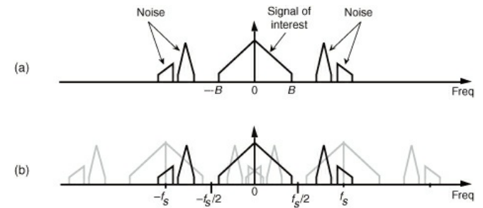
Noise in Bandpass Sampling
- Suppose that the signal has some noise outside the region of interest. The power of the noise of the sampled signal increases by a factor of (m+1) while the signal power remains the same. Hence, the Signal to Noise Ratio (SNR) decreases by this same factor
DFTs
- The continuous Fourier transform has the form $X(f) = \int_{-\infty}^{\infty} x(t) exp(-i 2\pi f t) dt$
- The discretized version looks like $X(m) = \Sigma_{n=0}^{N-1} x(n) exp(\frac{-i 2\pi nm}{N})$
- Remember that each m can be mapped to some frequency via $f(m) = \frac{m f_{s}}{N}$ where m ranges from 0 to N-1
- You can think of each X(m) as a point-for-point multiplication between the input values and some complex sinusoid
- The X(0) term simplifies to $X(0) = \Sigma_{n=0}^{N-1} x(n)$, which is just proportional to the average.
- This is the DC bias of the signal
- Occasionally, you will get some normalization term in front of the DFT
- The convention used here is to have a factor of $\frac{1}{N}$ on the inverse Fourier Transform
- Some code uses a factor of $\frac{1}{\sqrt{N}}$ for both the forward and inverse Fourier transform. The reasoning behind this is so that there is no scale change when transforming in either direction
DFT Properties
- Most signals that we care about are real. Under this assumption:
- $X(m) = X^{*}(N-m)
- If x(n) is even, then X(m) is real and even
- if x(n) is odd, then X(m) is imaginary and odd
- DFTs are linear transformations
- If you shift x(n) by k samples ,then the resulting DFT is shifted by an associated phase
- More concretely: $x(n) \rightarrow x(n+k)$ implies that $X_{shifted}(m) = exp(\frac{i 2\pi k m }{N}) X(m)$
DFT Leakage
- What happens if your signal doesn’t exactly equal a harmonic of $\frac{f_{s}}{N}$?
- The power of that frequency gets spread across all of the spectra (or all of the bins)
- This leakage means that bins which contain low-level signals get corrupted by high-amplitude signals in neighboring bins
- Another thing to note is that is leakage is periodic (ie. the m=0 bin can leak onto the N-1 bin)
Windows
- Leakage occurs due to the sidebands of the Fourier transform of the signal
- One way to mitigate this is via windowing
- For each datapoint in your Fourier transform, you add some weight to each sample
- Hence, the weighted Fourier transform becomes: $X_{w}(m) = \Sigma_{n=0}^{N-1} w(n) x(n) exp(\frac{-i 2\pi nm}{N})$
- You pick your weights such that the beginning and end of the sample interval both go smoothly to some common amplitude value
- There are a bunch of different weighting schemes:
- Boxcar/uniform/rectangular: $w(n) = 1$ for all n
- Triangular: $w(n) = \frac{n}{N/2}$ for n from 0 to N/2 and $w(n) = 2-\frac{n}{N/2}$ for N between N/2+1 to N-1
- Hanning: $w(n) = 0.5-0.5\cos(\frac{2\pi n}{N})$ for all n
- Hamming: $w(n)
- The standard Fourier transform uses boxcar. This results in a Fourier transform of sinc(x). The side lobes of sinc are due to the sharp edges of the sampling window. The alternative windowing functions try to smoothly taper off to 0 instead
- The trade-offs for having a reduced sideband response is that the mainband gets stretched out in frequency space
Scalloping
- For simplicity, assume no windowing (re: boxcar). Each Fourier bin gets transformed via sinc(x)
- The overlap between adjacent bins creates this ripple in the overall magnitude of the DFT away from the bin centers (see below for visual)
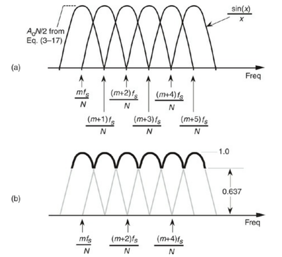
- In practice, this apparently isn’t a big problem, since most applications have so many frequency bins that this ripple is not noticeable
Zero-Padding
- The idea behind this is to inflate the number of sampled points by adding zeros to the end of a input
- This is typically done up to the nearest power of 2 for FFT reasons
- The net result of this is to get a better approximation of the CFT
- One side effect is that the index associated with each point gets changed as you zero pad
- This is not a bad thing, since the associated frequency of that bin is still the same as the original
- One gotcha that you might encounter is combining zero-padding and windowing. Make sure that your window doesn’t touch the zero-padding!
DFT Processing Gain
- Can think of each DFT bin as a bandpass filter centered around some frequency
- This bandpass effect can allow one to extract single frequencies from some background noise
- As the number of points increases, the signal frequency rises above the noise
- Can define a signal-to-noise ratio (SNR) which is the amplitude of the signal over the average background noise
- Increasing the number of points tends to increase the SNR
- Can’t increase ad infinitum because the number of multiplications scale as $N^{2}$
- An alternative approach is to average a smaller number of DFTs
DFTs in Practice
- Use some FFT implementation instead of the naive DFT
- Cooley-Tukey’s radix-2 is the classic version
- Make sure that you same fast enough and long enough
- fast enough means meeting Nyquist criterion at minimum (typical applications aim for 2.5x to 4x the bandwidth)
- If you don’t know the input frequency, watch out for FFT results which have large spectral components near half the sampling rate (re: aliasing)
- The number of samples you need to collect is given by $N = \frac{f_s}{f_{r}}$ where $f_{r}$ is your frequency resolution
- Make sure to round up to the nearest power of 2 for FFT reasons
- fast enough means meeting Nyquist criterion at minimum (typical applications aim for 2.5x to 4x the bandwidth)
- Make sure to zero pad your data as needed
- If you’re zero padding, make sure that you do this after windowing your signal
- Leakage is still a problem even if you zero pad
- the DC bias can affect your upper spectrum due to warping
- To mitigate this, can do an averaging of the time sequence and subtract of this average, removing the DC bias
- Make sure to do this before windowing
- To mitigate this, can do an averaging of the time sequence and subtract of this average, removing the DC bias
- the DC bias can affect your upper spectrum due to warping
- If you need to improve SNR, try taking multiple small FFTs and averaging them
- Apparently, this lets you detect signals which are buried in the noise?
Finite Impulse Response (FIR) Filters
- Given a finite duration of nonzero input values, an FIR filter wil eventually output a finite duration of of nonzero output values
- Conversely, if the input to an FIR filter suddenly became all zeros, the output would eventually become all zeros
- Can think of averaging as a simple example of an FIR filter that demonstrates the above:
- If the input signal suddenly drops to zero, the average will gradually taper off to zero
- Can be thought of as a kind of low pass filter
- The “delay” modules can be though of as shift registers which temporarily store the values for the computation
- Due to these delay modules, any change in the input takes some time to be realized in the output. The intermediate output of the filter is called the “transient” period
FIRs as Convolution
- Picture a general M-tap FIR filter. The nth output is then $y(n) = \Sigma_{k=0}^{M-1} h(k) x(n-k)$ where $h(k)$ is the weight which gets applies to the kth input. This is the definition of a convolution
- Using the convolution theorem, we can equal convolution in the time domain to multiplication in the frequency domain
- (ie $h(n) * x(n) = H(m) \times X(m)$, where * denotes the convolution)
- One way to determine h(k) is to send an impulse response as input, then see what the filter outputs
- Can take the Fourier transform of the above to get H(m)
Lowpass FIR Filter Design
- What if we want to go the other way around? Given some cutoff frequency, what coefficients do we need to implement a lowpass FIR filter?
- There are two methods to figure out the coefficients: window design, and optimum methods
- For simplicity, assume a perfect low pass filter: unity gain below the threshold frequency, and zero gain above the threshold
Window Design
- Take the inverse Fourier transform of your desired frequency response in order to get the coefficients
- Some nuances:
- you want to define the frequency response from 0 to $f_{s}$ instead of the symmetric $\mp \frac{f_{s}}{2}$
- When you do this process, you get some ripple power in your reconstructed filter due to Gibb’s phenomena
- This arises because no finite set of sinuoids will be able to change fast enough to be equal to an instantaneous discontinuity
- If you’re doing windowing, there is a trade off between ripple power suppression and main lobe widening that you need to figure out
- Two windows which allow a fine-tuning of this trade off are the Chebyshev window and the Kaiser window
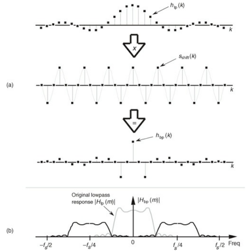
Bandpass and High Pass Design
- Due to the negative frequencies, a “low pass” filter is roughly symmetric around the origin
- If you could shift this band up so that it’s centered at $\frac{f_{s}}{4}$, then you would get a bandpass filter around $\frac{f_{s}}{4}$!
- This can be achieved by multiplying you low pass filter coefficients by a sinusoid of frequency $\frac{f_{s}}{4}$
- This takes the form of a sequence ${-1,0,1,0,-1,…}$
- A high pass filter is analogous, but you instead multiply by by a sinusoid of frequency $\frac{f_{s}}{2}$
- This takes the form of a sequence ${-1,1,-1,…}$
Parks-McClellan Exchange FIR Filter Design Method (Optimum Method)
- In one sentence, Parks-McClellan tries to minimize the error in the pass and stop bands by utilizing the Chebyshev approximation
- It’s the defacto FIR filter generation algorithm and can be used for most realistic response curves
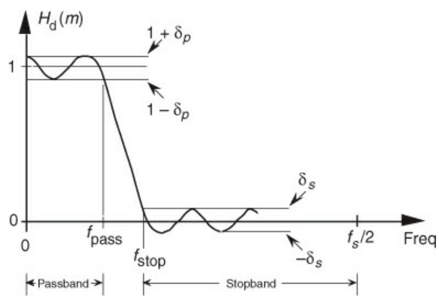
- We define $f_{p}$ and $f_{s}$ as the upper frequency bound on the low pass side and the lower frequency bound on the stop band side
- We also define $\delta_{p}$ and $\delta_{s}$ as the ripple deviation in the low pass and stop bands
Half-Band Filters
- The basic idea here is that we want the frequency response to be symmetric around $\frac{f_{s}}{4}$
- This implies that the average of $f_{p}$ and $f{s}$ is $\frac{f_{s}}{4}$
- If the number of coefficients is odd, then every other coefficient is zero (excluding the central tap)
- This halves the number of multiplications needed to do the filter
- The number of taps N must be such that N+1 is a multiple of 4. Otherwise, you reduce down to a smaller effective number of taps
- You can use the Optimum Method to generate Half-Band filters of this type
FIR Filter Phase Considerations
- We need to introduce the idea of group delay. Think of it as $G = -\frac{d\phi}{df}$ where $\phi$ is the phase
- We want G constant for amplitude modulated (AM) signals
- Why? Because if G is constant, all of the frequency components get delayed by the same amount. This ensure that the shape of the incident wave packet is conserved
- We want G constant for amplitude modulated (AM) signals
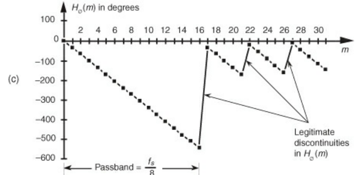
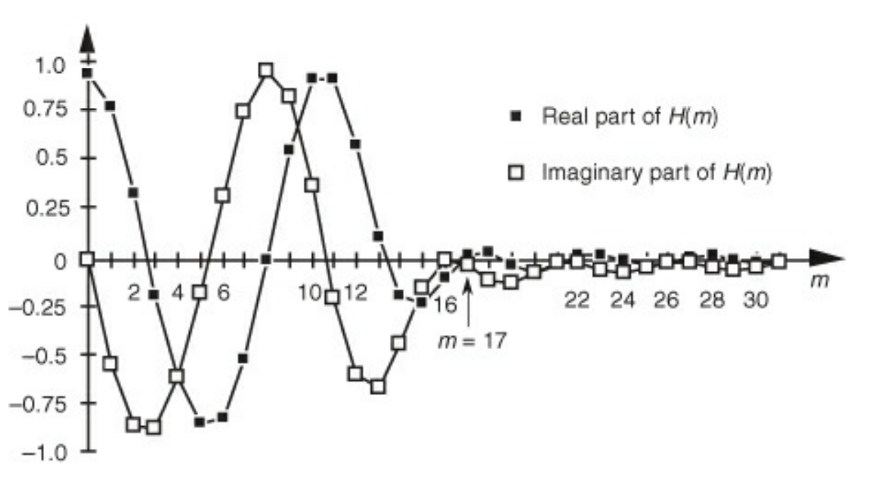
- There are two ways in which discontinuities can show up in a phase response plot
- the range of arctan is $-\frac{\pi}{2}$ to $\frac{\pi}{2}$. Lots of software will force results to lie within this region. This is not physical
- Remember that the phase response function is complex. For each frequency component of the response, if the polarity of one component changes while the other remains the same, then a jump discontinuity will occur. This is physical
Infinite Impulse Response (IIR) Filters
- IIR Filters allow feedback from their output
- Think of FIR filters as Moore FSMs, and IIR filters as Mealy FSMs
- The “Infinite” comes from the fact that you can end up in a state where the filter continuously outputs stuff even if there is no input
- Why use IIRs?
- Because they can be more efficient that FIRs (re: fewer multiplications), which allows higher sampling rates compared to FIRs
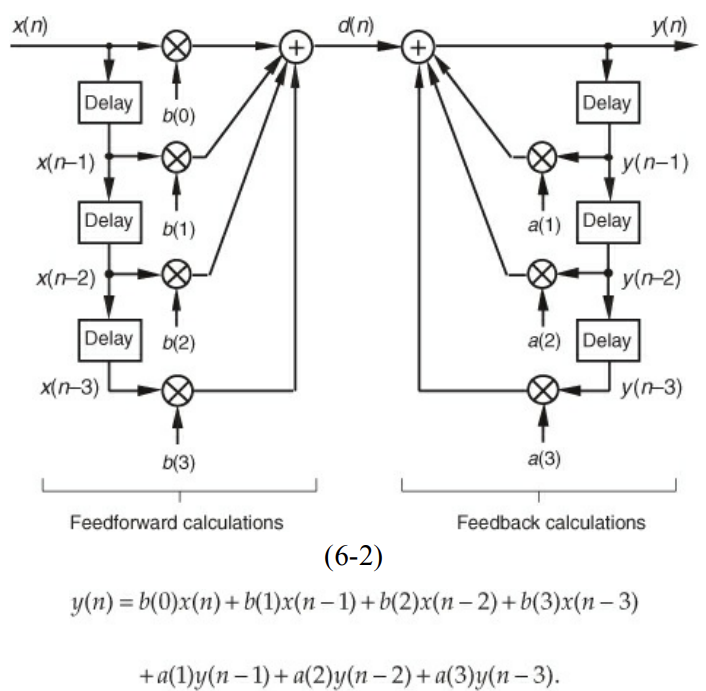
- IIRs consist of feedforward coefficients $b(k)$ (like an FIR filter) and feedback coefficients $a(k)$, which couple past outputs to the current on
- You can’t calculate the IIR coefficients from the impulse response (not even $b(k)$!)
Laplace Transforms
- Useful tool for solving differential equations
- Take Laplace transform, do algebra to get output function’s form in Laplace domain, and then inverse Laplace transform
- Defined as $F(s) = \int_{0}^{\infty} f(t) e^{-st} dt$ where s is a complex number: $s = \sigma+\omega i$, which can be though of as a complex frequency
- The Laplace transform allows you to convert the time series of the inputs and outputs into the complex frequency space ($X(s)$ and $Y(s)$ respectively)
- The transformation which enables you to go from $X(s)$ to $Y(s)$ is called the transfer function $H(s)$ ie. $Y(s) = H(s) X(s)$
- In principle, given a transfer function, one can Laplace transform x(t), apply H(s), then inverse Laplace to get y(t)
- In practice, H(s) have enough information to give you the frequency response as well as if the filter is stable
Stability
- TL;DR look at the poles of H(s)
- What are poles? They are complex numbers $s_{0}$ where the transfer functions blows up
- They are called poles because if you look at the magnitude of H(s) around $s_{0}$, it looks like a flag pole
- H(s) can have multiple poles
- Let $s_{0} = \sigma_{0}+\omega_{0} i$ be a pole of H(s). If $\sigma_{0}$ is positive, the system is unstable. If $\sigma_{0}=0$, then the system is conditionally unstable (re. it will oscillate back and forth)
- There are also zeros of H(s), which correspond to the numerator beinng zero
- People typically denote “x” for poles and “o” for zeros on the complex plane
Z-Transform
- This is a discretized version of the Laplace transform that can be used to construct IIR filters
- Continuous Laplace equations get applied to differential equations, while the z-transform gets applied to difference equations
- It’s defined as $H(z) = \Sigma_{n=-\infty}^{\infty} h(n) z^{-n}$
- If we write z in polar form: $H(z) = \Sigma_{n=-\infty}^{\infty} h(n) r^{-n} exp(-i\omega n)$
- From the r term, we immediately see that the stability condition is that $|z| \leq 1$
- The ranges of frequencies are also restricted by the sampling frequency (ie. $\frac{\omega_{s}}{2} \geq \omega \geq \frac{-\omega_{s}}{2}$)
- Hence, if all of the poles of a transfer function are located inside the unit circle, things are stable
- Adding a delay in your signal processing pipeline looks like $y(n) = x(n-1)$
- Plugging that into the z-transform, changing variables to $k=n-1$ and rearranging, you get that $Y(z) = z^{-1} X(z)$
- or more verbosely, having k delay units multiplies the Z transform by $z^{-k}$
- Alternatively, a transfer funtion of $z^{-k}$ can be thought of as a delay of $kt_{s}$ seconds where $t_{s} = \frac{1}{f_{s}}$
Applications to IIR
- We can write any M-th order IIR filter with N feedforward states and M feedback stages in Direct Form I
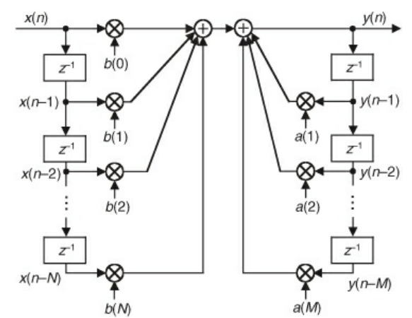
- We can write the output Z-transform as:
- $Y(z) = X(z) \Sigma_{k=0}^{N} b(k) z^{-k} + Y(z) \Sigma_{k=1}^{M} a(k) z^{-k}$
- We can then define the transfer function as $H(z) = \frac{Y(z)}{X(z)} = \frac{\Sigma_{k=0}^{N} b(k) z^{-k}}{1-\Sigma_{k=1}^{M} a(k) z^{-k}}$
- The order of the transfer function is the larger of M or N
- You can make the substitution $z = e^{i\omega}$ (remember, stability means that the radius is 1!) to get the frequency response
- This can be though of as taking the intersection of the unit radius cylinder with $H(\omega)$, cutting the curve at the $\pi$ branch cut and then unwrapping everything
Various Notations for IIR Filters

- For simplicity, assume that M and N are equal (same number of feedforward and feedbackwards stages)
- Since everything is linear and time invariant, we have some freedom to shuffle around the multiplications and additions
Transposition Theorem
- To transpose a filter:
- Reverse the direction of all signal-flow arrows
- Convert all adders to signal nodes
- Convert all signal nodes to adders
- Swap the x(n) input and y(n) output labels
- Why would you do this?
- Say you’re transposing Direct Form I. The transpose first calculates the zeros, then the poles. The poles can lead to a blowup in intermediate calculations, so postponing this calculation until the end helps prevent truncation
Finite Precision Effects in IIRs
- Since we can’t use infinite precision arithmetic, we need to used a finite precision representation of all of our computation
- The three major problems from this discretization are:
- Coefficient quantization: Lacking the necessary precision on coefficients causes the zeros and poles to wobble around, which can result in stability issues and a distorted frequency response
- Overflow errors: Intermediate calculations can go outside the dynamic range of the precision specified. This can lead to overflow oscillations
- Roundoff errors: To mitigate the overflow issues, you can round off intermediate calculations to some specified precision
- You can normally treat roundoff errors as some random process
- The roundoff noise becomes highly correlated with the signal (called limit cycles). This can cause infinite oscillations
Chaining Filters Together
- If you cascade one filter after another, then overall transfer function of the system is the product of the two
- The associated coefficients are also the convolution of the two original filters
- If you run two filters in parallel with each other (ie. same inputs) then sum their outputs, the overall transfer function is the sum of the two individual transfer functions
- The coefficients are simply the sum of the two original filters
- This idea allows you to break down a higher order filter into smaller order ones, which are easier to work with
- One big problem is a combinatorial explosion of equivalent circuits (assuming infinite precision)
- To demonstrate this, say you want to break down a 2M order filter into M distinct 2nd-order filters there are M! ways of arranging these filters, and there are M! ways of pairing coefficients of the filters
- If you’re dealing with 2nd order filters, there is a simple (but not-optimal) algorithm to make these choices:
- First, factor a high-order IIR filter into the form $H(z) = \frac{\Sigma_{i}^{N} (z-z_{i})}{\Sigma_{j}^{N} (z-p_{i})^}$ where N denotes the number of poles and zeros
- After than, find a pole or pole pair closest to the unit circle, then find the zero which is closest to those poles. These poles and zeros form one of your 2nd order filters. Remove them from the pool, repeat this procedure until nothing is left
Scaling Gain of IIR Filters
- For some applications, we want to be able to limit the gain of the data values in the IIR filter
- This is accomplished by modifying the DC gain of the filter
- The DC gain is defined as $\frac{\Sigma b(k)}{1-\Sigma a(k)}$ or in words: the sume of the feedforward coefficients divided by 1 minus the sum of the feedback coefficients
- If we want to have a DC gain of 1, we simply divide all of the coefficients by this initial DC gain
- Neither the frequency response nor the phase response does not change
Differentiators, Integrators, and Matched Filters
Differentiators
- Imagine a continuous analog sine wave. It’s derivative is a cosine times the angular frequency
- The transfer function of the ideal differentiator is $H(\omega) = i \omega$
- Can easily derive by taking the Fourier transform of derivative of signal
- The transfer function of the ideal differentiator is $H(\omega) = i \omega$
- The naive way of implementing this is via a tapped-delay line structure
- A First difference differentiator simply subtracts adjacent sames from each other
- The First difference method is very sensitive to noise and high frequency signals
- This follows from the frequency response of the filter: $|H(\omega)| = 2 |\sin (\frac{\omega}{2})|$
- The First difference method is very sensitive to noise and high frequency signals
- A Central-difference differentiator takes the average of two consecutive first difference differentiators
- This works out to $\frac{x(n)-x(n-2)}{2}$
- The central difference method is more robust against noise, but there is the linear regime is smaller than that of the finite difference method
- Follows from $|H(\omega)| = |\sin (\omega)|$
- Both of these methods have a very narrow operating regime. Which means that you can only use these if the input has a low spectral content compared to the sampling rate
- The group delay of both of these filters goes like $\frac{D}{2}$ where D is the number of taps involved
- This follows from the anti-symmetry in the coefficients
- Weather the delay is an integer or not is important for specific applications
- A First difference differentiator simply subtracts adjacent sames from each other
- In practice, you shove the frequency response through Park-McClellan to get the best performing filter
- Oddly enough, you get a more accurate differentiation when N is even compared to when N is odd
- You can also window the input sequence to reduce the ripples in frequency space
Narrowband Differentiators
- Richard Hamming proposed a family of low-noise Lanczos differentiating filters, which have 2M+1 coefficients
- You generate the coefficients via $h(k) = \frac{-3k}{M(M+1)(2M+1)}$ where k ranges from -M to M
- This has a smaller linear operating frequency range compared to the naive way
- You can implement this filter with half the multiplications as the number of taps
- You can also multiply through by the common denominator in order to do integer multiplication instead of floating point
Wideband Differentiators
- Suppose that we want to be able to differentiate a large number of frequencies up to some cutoff $\omega_{c}$, after which we have perfect attenuation
- This is impossible to do without an infinite number of taps
- All approximations will have some ripples at frequencies above the cutoff
- Taking the inverse transform of the ideal frequency response yields $h_{gen}(k) = \frac{\omega_{c}\cos(\omega_{c}k)}{\pi k} - \frac{\omega_{c}\sin(\omega_{c}k)}{\pi k^{2}}$
- This is sufficient, but it has negatives, which are annoying to work with
- We can rewrite the coefficients as $h_{gen}(k) = \frac{\omega_{c} \cos(\omega_{c} \lceil k-M\rceil)}{\pi \lceil k-M\rceil}-\frac{\omega_{c} \sin(\omega_{c} \lceil k-M\rceil)}{\pi \lceil k-M\rceil^{2}}$
- $M = \frac{N-1}{2}$ and $0 \leq k \leq N-1$
- We can rewrite the coefficients as $h_{gen}(k) = \frac{\omega_{c} \cos(\omega_{c} \lceil k-M\rceil)}{\pi \lceil k-M\rceil}-\frac{\omega_{c} \sin(\omega_{c} \lceil k-M\rceil)}{\pi \lceil k-M\rceil^{2}}$
Integrators
- An ideal analog integrator has a frequency response proportional to $\frac{1}{\omega}$
- Discretization prevents us from doing this, but there are several schemes which approximate this
- Rectangular Rule: Simply keep a running sum of all of the inputs
- $y_{Re}(n) = x(n) + y_{Re}(n-1)$
- $H_{Re}(\omega) = \frac{1}{1-exp(-i\omega)}$
- Trapezoidal Rule: Average the two most recent incoming signals
- $y_{Tr}(n) = 0.5 x(n) + 0.5 x(n-1) + y_{Tr}(n-1)$
- $H_{Tr}(\omega) = \frac{0.5+0.5exp(-i\omega)}{1-exp(-i \omega)}$
- Simpson’s Rule: Weight the three most recent incoming signals as though you fit a quadratic to them
- $y_{Si}(n) = \frac{x(n)+4x(n-1)+x(n-2)}{3} + y_{Si}(n-2)$
- $H_{Si}(\omega) = \frac{1+4 exp(-i\omega)+exp(-2\omega i)}{3(1-exp(-2i \omega))}$
- All of the above have z-domain transfer function poles at z=1, which corresponds to a cyclic frequency of 0
- This means that the register widths need to be large enough to prevent overflow from corrupting an integrator

- The above shows the absolute error of each of the integrators
- Tick’s rule is some weird scheme which trades off drastically larger errors at high frequencies for more precise low frequency approximation
Matched Filters
- Suppose that our input consists of a signal component and a noise component
- We want the filter to be able to output the signal to noise ratio (SNR), which can then be passed to some thresholding function to determine if a signal of interest was detected
- The design goal of the filter is to maximize the SNR
- For an analog signal, the optimum frequency response is $H(f) = S(f)^{\dag}e^{-2\pi f T i}$ where $\dag$ refers to complex conjugation and T is the time duration of the signal
- Physically, this is the complex conjugate of the frequency response times a linear phase shift which is proportional to T
- Can think of this as convolution: you have some reference template which you drag across the input signal. The maximum SNR occurs when the dot product is minimized
- Physically, the phase of the signal constructively interferes when the input matches the template, but the noise destructively interferes
- We can discretize under the following assumptions:
- The signal of interest is some N sample sequence
- $S(m)$ is the N-point DFT of the signal of interest
- m is some discrete frequency index $0 \leq m \leq N-1$
- $x_{in}$ is sampled at a rate of $f_{s}$
- The time of the N-length sample sequence is N-1 sample periods
- Hence we get $H(m) = S^{\dag}(m) exp(-\frac{2\pi m (N-1)}{N}i)$
- the associated coefficients are $h(k) = x_{s}(N-k-1)$ where $0 \leq k \leq N-1$
- A matched filter can be thought of as a digital correlator
- If the samplings are large, it may be more efficient to do multiplication in frequency domain than convolution in time domain
Quadrature Signals
- What if, instead of a real signal, you have a complex signal?
- This complex signal is called a quadrature signal, and takes the form $e^{i 2\pi f t} = cos(2\pi f t) + i sin (2\pi f t)$
- You can generate an “imaginary” signal via multiplication by i: delay the phase of the input by $\frac{\pi}{2}$
- In order to generate a quadrature, you could have two function generators which generate cosine and sine respectively. As long as you keep the phase delay between the two pinned to $\frac{\pi}{2}$, then the two wires together are a quadrature
- Hence, you always need two wires to represent a quadrature
- This complex signal is called a quadrature signal, and takes the form $e^{i 2\pi f t} = cos(2\pi f t) + i sin (2\pi f t)$
- Can imagine two classes of quadrature signals in the complex plane. One rotates clockwise, while the other goes counter-clockwise
- This gives rise to the notion of “negative frequencies”. They are simply signals which have the opposite polarization as the standard signals
- If you are representing a real signal in quadrature, the negative and positive frequencies are evenly symmetric around the DC point
- Similarly, purely imaginary signals have odd symmetry around the DC point
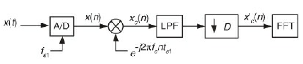
Down Conversion
- Imagine that you have some real-valued time sequence x(n). This has a corresponding frequency representation which is symmetric around f=0 and is joined at $\frac{f_{s}}{2}$
- If we multiply x(n) by $e^{-i 2\pi f_{c} n t_{s}}$, where $t_{s} = \frac{1}{f_{s}}$ and $f_{c}$ is some frequency shift less than $f_{s}$, then we have effectively shifted the spectra over by $f_{c}$
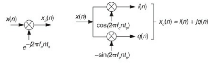
- This multiplication involves splitting up the signal and multiplying each branch by cosine and negative sine respectively
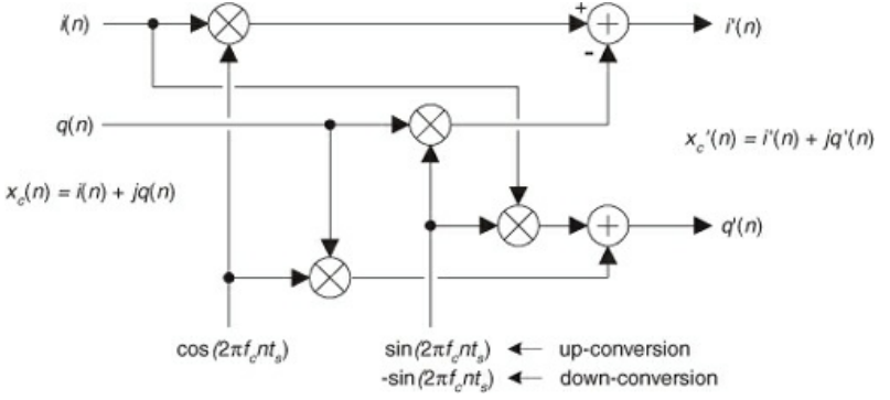
- An analogous construction holds for quadrature signals
- One big sticking point of this type of down conversion is that there needs to be a very strict 90 phase delay between the wires of the quadrature signal
- If you digitize before you do the mixing, this helps lock the phase difference
Complex Resonators
- You can think of the above IIR filter as a way of generating a frequency between 0 and $f_{s}$ Hz
- If you let x(n) be a unity impulse (re 1, then 0 forever after), this circuit will oscillate at a rate specified by $\omega_{r}$
- $\omega_{r}$ is a normalized angle between 0 and $2\pi$
- So if you want $\frac{f_{s}}{4}$ as the output frequency, set $\omega_{r} = \frac{\pi}{2}$ and take the real component of the output
- If you let x(n) be a unity impulse (re 1, then 0 forever after), this circuit will oscillate at a rate specified by $\omega_{r}$
Hilbert Transform
- The Hilbert transformation let’s you convert real signals to complex signals
- Can think of this as multiplication by i. In physical terms, this is a 90 degree phase delay. This can be combined with the original signal to produce a quadrature signal
- So we need to design a circuit which, given a purely real input signal, outputs the same signal, but delays by 90 degrees
- What is the frequency response of the shifted output?
- $X_{ht}(\omega) = H(\omega) X_{r}(\omega)$
- $H(\omega) = \pm i $ where -i is over positive frequencies and +i is over negative frequencies
- Suppose that you can perform the Hilbert transform on $x_{r}$. The Fourier transform of the quadrature signal is $X_{c}(\omega) = X_{r}(\omega)+ i X_{i}(\omega)$
- This is zero in the negative frequencies (ie. a one sided signal)
Impulse Response for Hilbert Transform
- We know what the response function in frequency space looks like: $H(\omega) = \pm i $
- Taking the inverse Fourier transform yields: $h(t) = \frac{1-cos(\frac{\omega_{s} t}{2})}{\pi t}$ where $\omega_{s} = 2\pi f_{s}$
- This can be digitized to $h(n) = \frac{f_{s}}{\pi n}(1-cos(\pi n))$
- For $n=0$, let $h(n)=0$
- This can be digitized to $h(n) = \frac{f_{s}}{\pi n}(1-cos(\pi n))$
FIR Implementation
- Naively, we could simply just use the h(n) coefficients and convolve them with the incoming time sequence. Little problem: there are an infinite number of coefficients, so we need to truncate the series
- If the truncation as an odd number of taps and the coefficients are antisymmetric (as in the case of the Hilbert transform), $|H(0)| = 0$ and $|H(\frac{\omega_{s}}{2})| = 0$. If there are an even number of taps, only the DC component of H needs to be 0
- Look at the above 15 tap Hilbert transform above
- The magnitude response drops off at 0. This effectively turns the Hilbert transform into a bandpass filter
- There is some ripple in the passband. This comes from the finite number of taps in the coefficients. You can reduce the ripple via windowing, but this will reduce the bandwidth of the filter
- Due to the aforementioned drop off, it’s hard to compute the Hilbert Transform of low-frequency signals
- The phase response is linear (with a slight discontinuity at 0)
- To offset this phase response, we delay the real component of the quadrature signal by the group delay (which remember, is $G = \frac{D}{2}$ where D is the number of delay elements)
- Given a set of coefficients, remember to reverse the order in order to do the convolution. For most FIR filters, the coefficients are symmetric, so this doesn’t matter, but Hilbert filters aren’t
Sample Rate Conversion
- Say that you have two hardware processors operating at two different sample rates. You need to exchange data between the two. How do you do this?
- One way this could be done is to do use a DAC and ADC setup to convert to an analog signal, then resample at the new rate. This limits the dynamic range of the signal and is not normally utilized
- What you do depends if you are increase the sample rate or decrease the sample rate
- As an aside, people in the DSP community use a lot of similar sounding words to describe various concepts of sampling rate conversion
- Use the above to make the transition between terms
Decimation
- Decimation is how you go about downsampling. It consists of low pass filtering a signal, and then downsampling
- Downsampling by a factor of M is done by only keeping every Mth sample, then discarding the rest. This reduces the sampling rate by a factor of M
- Care needs to be taken to ensure that the new sampling rate still obeys the Nyquist criterion (ie. the sampling rate is twice the bandwidth of the signal), otherwise aliasing can occur
- The lowpass portion is essential when you drop below the Nyquist limit (ie. it prevents the upper frequencies of your signal from aliasing with the lower frequencies)
- The low pass portion of decimation can most easily be done with a FIR filter (due to the linear phase response)
Two-Stage Decimation
- It may be more computationally efficient and stable to break a decimation block into multiple sub-blocks
- Ie. The number of taps that you is can be significantly lower than a single stage
- If you have two stage decimation (so the downsampling factor is $M = M_{1}M_{2}$), the optimal value for $M_{1}$ becomes:
- $M_{opt} = 2M \frac{1-\sqrt{\frac{MF}{2-F}}}{2-F(M+1)}$
- $F = \frac{f_{stop}-B}{f_{stop}}$
- This is the ratio of the single-stage low pass filter’s transition region width to that of the filter’s stopband frequency
Downsampling Gotchas
- Downsampling is not a time invariant process. So you aren’t allowed to reorder time invariant operations with it
- While downsampling doesn’t cause time-domain signal amplitude loss, there is a drop in magnitude by a factor of M in the frequency domain
Interpolation
- Interpolation can be thought of as upsampling, followed by a low pass filter
- Upsampling by a factor of L can be thought of as inserting L-1 samples between each of the original signal’s samples
- One easy way of upsampling is via zero stuffing: make all of the new intermediate values 0!
- You then need to lowpass filter this interpolated signal to smooth the signal
- Another potential way of interpolating is just to repeat the values of the original sequence until the next one
- The problem with this is that the frequency domain gets multiplied by a sinc function. This would require an egregious number of taps in the lowpass filter to smooth out
Interpolation Gotchas
- An artifact of upsampling is that, in frequency space, you get phantom copies of the original spectra. An ideal lowpass would eliminate these copies completely, but due to the attenuation of real filters, there is always some residue
- Due to the zeros, the interpolation reduces the time series magnitude by a factor of L. You need a corresponding DC offset of L to maintain a unity transformation
- Conversely, the frequency magnitude will increase by a factor of L
Polyphase Filters
- Naively, if you want a sampling rate that this not an integer, then you would need to chain decimations and interpolations of different integers
- Doing this by zero padding and discarding samples is excessively wasteful
- Polyphase filters helps eliminate this unnecessary computation
Polyphase Interpolation and Decimation
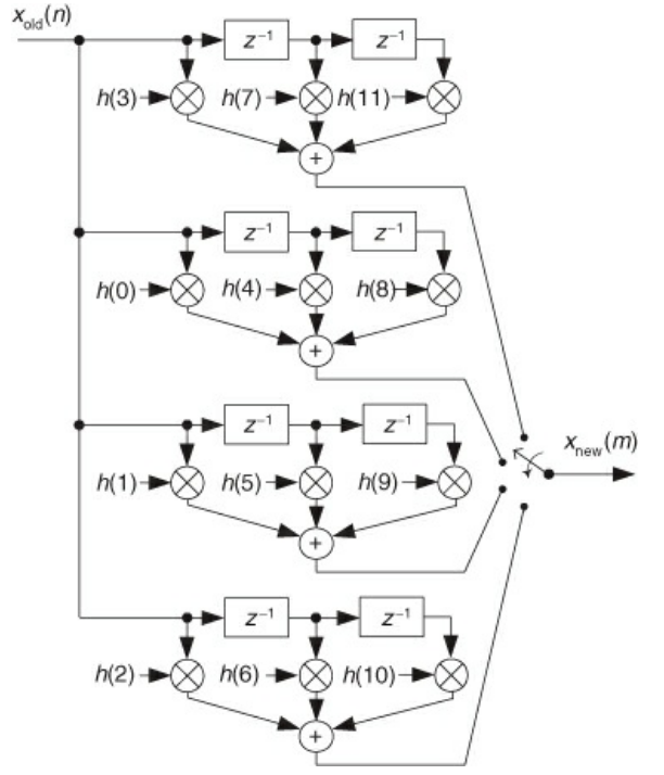
- Interpolation is easier to understand. Suppose that you have a 12-tap low pass filter and you want to upsample by a factor of 4
- For x(0), there are only three meaningful multiplications; the rest get zeroed out
- For x(1) (re: the next sample over), there are still only three meaningful multiplications; the difference is that the FIR coefficients you are using are all different
- This repeats for x(2) and x(3)
- If you perform all of these branches in parallel, and then multiplex the output based on the current sample, then you have effectively eliminated all of the zeroing
- The implementation shown in the image above is not really any more efficient than the zeroing scheme (3 out of the 4 branches are just getting wasted)
- Instead of multiplexing the output, you can multiplex the coefficients instead. This way, only one branch is active at a given time
- Some gotchas:
- Try and make sure that the initial FIR filter has an integer multiple of your interpolation factor for ease of implementation
- Polyphase interpolation still has drops in magnitude by a factor of L
- Can fix by scaling the coefficients by L, or multiplying the output by L
- Decimation is very similar
- In fact, you use the same FIR coefficients as interpolation!
- Now, instead of multiplexing the output, you multiplex your input down each branch sequentially, then sum the outputs of all the branches
- The z-transformation of a up/downsampled signal is simply
- $W(z) = X(z^{L})$ for upsampling and $W(z) = X(z^{\frac{1}{L}})$ for downsampling
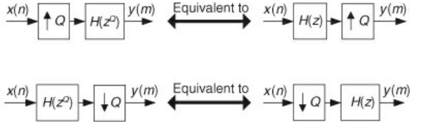
- Because upsampling and downsampling are not time invariant, you can’t swap them around with other filters arbitrarily
- However, if the filters have some special form, then it’s alright
- Specifically, you can swap a transfer function of the form $H(z^{L})$ witth an upsampler and downsampler as per the noble identities
Cascaded Integrator Comb (CIC) Filters
- CIC filters are computationally efficient implementations of narrowband lowpass filters
- Very useful for anti-aliasing filtering in decimation and interpolation
- A key advantage of these filters is that they require only additions and subtractions
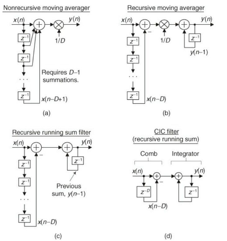
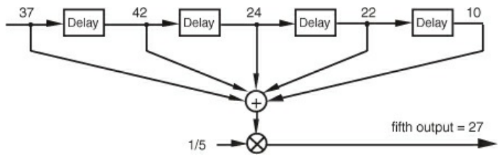
- The above image shows D point moving averagers
- A running sum is an averager that doesn’t do the one multiplication
- Fig a shows a standard non-recursive averager
- Fig b shows an equivalent recursive setup: instead of summing all of the delayed elements, you delay the signal by D cycles, then subtract that from the input, multiply by 1/D, and then add the last sample
- Fig c is equivalent to Fig b, but without the multiplication
- Fig d is equivalent to Fig c, but uses more compact notation for the delay elements and annotates each section
- The governing difference equation of Fig. d is
- $y(n) = x(n)-x(n-D)+y(n-1)$
- The feedforward section (re $x(n)-x(n-D)$) is the comb section, the delay unit is called differential delay, and the feedback section is called the integrator
- The associated transfer function is then $H(z) = \frac{1-z^{D}}{1-z^{-1}}$
- The corresponding frequency response is $H(f) = exp(-i\pi f(D-1)) \frac{\sin(\pi f D)}{\sin(\pi f)}$
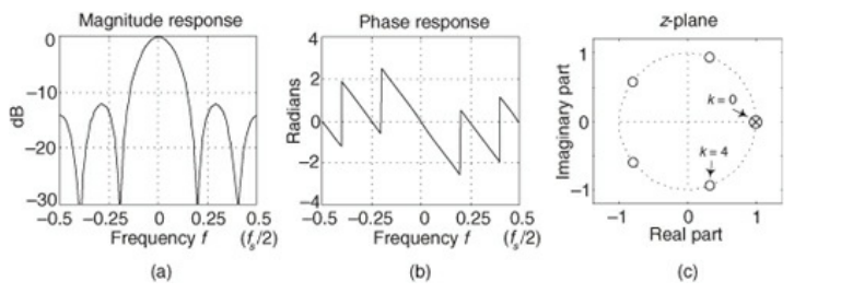
- The above shows the characteristics of a D=5 CIC filter
- The magnitude of the frequency response is like a squared sinc function
- The phase response is piecewise linear, with jump discontinuities at the crossing points of the frequency magnitudes
- There is a pole on the edge of the unit circle, which ostensibly should lead to conditional stability. However, since there is no coefficient quantization error, this gives guaranteed stability to CIC filters
- The DC gain of the filter is D (use L’Hopital’s rule on frequency response at f=0)
Signal Averaging
- Can think of the mean, standard deviation, and variance of a set of N samples as the DC signal, the AC signal, and the power of the AC signal
- All of these involve calculating the mean of a signal. How do you do that?
Coherent Averaging
- An alternative name for this is time-synchronous averaging. This means that the start of each sample set is taken at the same phase of the target signal
- Take for instance, a sine wave with some noise on it. If the sine wave samples all start at the same phase, they will converge to the true sample, while the noise, which is decoherent, will go to zero
- This sort of averaging across a set of samples yields a SNR increase of $\sqrt{N}$, where $SNR = \frac{R}{\sigma}$
Incoherent Averaging
- This means that the start of each set of samples is not taken at phase (think of a oscilloscope without a proper trigger getting set)
- This is useless in the time-domain, but pretty useful in the frequency domain
- One particular application is a spectrum analyzer
- You want to figure out the spectra of a signal, but you don’t want a large tap DFT. Since addition is cheaper than multiplication, you can just take the average of multiple smaller DFTS
- You get a similar increase in SNR of the power measurements. This gain of SNR is called integration gain
Averaging Multiple DFTs
- Suppose that you have k DFTs, each with N taps
- Simply average across all of the k bins
- You get a reduction of the noise by a factor of k
- In practice, there is an overlap between adjacent DFTs (so points in the first DFT also show up in the second DFT etc.)
- How much overlap is too much? Keep it less than 50% and you don’t see any noticable reduction in SNR
Phase Averaging
- This is harder than time-domain signal averaging and frequency domain magnitude averaging due to the branch cut
- Treat the phase angles as the arguments of two complex numbers, add the numbers, then extract out the phase
Averaging Implementations
- You can use the standard moving averager discussed in previous sections, in both the recursive and non-recursive setup
- The problem with these are that N (the number of sample sets) must be an integer
- The second is that abrupt amplitude changes in the input don’t result in abrupt changes in the output (lowpass filter behavior and all that…)
- One popular averaging scheme is exponential averaging
- Define the recursive lowpass filter: $y(n) = \alpha x(n) + (1-\alpha) y(n-1)$ where $0 < \alpha < 1$
- There are three big benefits of this type of averaging:
- You can tune the frequency response of the filter by changing $\alpha$
- It requires less computation than the standard moving averager
- You only need one delay element
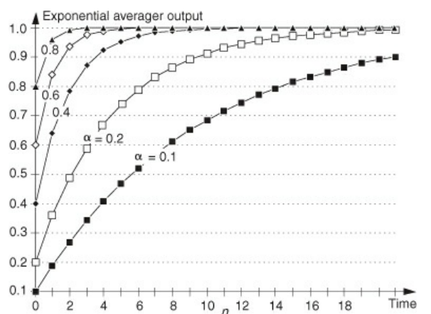
- The above shows the response of the exponential averager when the input is a step function
- If $\alpha$ is 1, then the input is not attenuated at all and no averaging takes place
- This makes it so that the averager responds immediately to changes in the input
- As $\alpha$ decreases, the response time of the filter also increases. The expoential weighting of previous inputs averages the signal and reduces noise
- A trick people use is to have a large $\alpha$ value initially so that there is an immediate output, then taper $\alpha$ off to increase SNR
- Given a certain noise reduction factor R, we can determine what $\alpha$ we need via: $\alpha = \frac{2}{R+1}$
- The frequency response has a pole at $z=1-\alpha$, so this is unconditionally stable
- The phase of this filter is nonlinear. We normally don’t care about this since averagers are more concerned with the DC response
- If $\alpha$ is 1, then the input is not attenuated at all and no averaging takes place
Digital Signal Processing Tricks
Frequency Translation by $\frac{f_{s}}{2}$
- Multiply x(n) by the sequence $(-1)^{n}$, where both sequences are run at $f_{s}$ sampling rate
- This is efficient since you don’t actually need to do multiplication; just flip the sign bit
- This can be shown by doing the convolution theorem
- use the form $(-1)^{n} = exp(i\pi n)$
- End effect is to shift the top and bottom halves of the spectra down and up (respectively) by a factor of $\frac{f_{s}}{2}$
Frequency Translation by $-\frac{f_{s}}{4}$
- Define the sequences
- $\cos(\frac{\pi n }{2}) = 1, 0, -1, 0, …$
- $\sin(\frac{\pi n}{2} ) = 0, -1, 0, 1, …$
- You can multiply these sequences with any x(n) to shift the frequency spectrum by $\frac{f_{s}{4}$ (sign depends on initial phase of cosine and sine sequences)
- Don’t acutally need multiplication, just sign flips and zeroing out
- The only difference between the outputs is the 90 degree phase shift
- Can use this to generate quadrature signal
High Speed Vector Magnitude Approximation $(\alpha Max + \beta Min$)
- Suppose that $I^{2}$ and $Q^{2}$ (representing the in-phase and quadrature signal powers) are readily available. How do you quickly calculate the square root of the sum of the two?
- A decent approximation is $|V| \approx \alpha Max + \beta Min$, where max and min are the larger and smaller of I and Q
- Can quickly compare magnitudes by dropping sign bit and comparing values
- If $\alpha$ and $\beta$ are both 1, this is just another way of writing the triangle inequality
- $\alpha$ and $\beta$ are typically chosen to be powers of two for easy multiplication, but not a hard restriction
- Need to experimentally determine optimal hyperparameters
- The error is dependent on the relative magnitude (re: phase) between I and Q
Conditional Faster Complex Multiplication
- In the very specific case where the hardware allows 3 addition operations to be faster than 1 multilplication, you can do complex multiplication faster by computing some intermediate values
- Define $k_{1} = a(c+d)$, $k_{2} = d(a+b)$, and $k_{3} = c(b-a)$ where a+ib and c+id are your two complex numbers
- then $R = k_{1} - k_{2}$ and $I = k_{1} + k_{3}$
- This takes 3 multiplications and 5 additions instead of 4 multiplications and 2 additions
Working with Real-Valued Data for FFTs
- The general FFT algorithm accepts complex numbers. Most data is real. You can trim the fat of the FFT to take advantage of this
- One way is to do the FFT of two seperate real sequences at the same time
- Suppose that you have two N point input sequences. Treat one sequence (a) as the real component, and the other (b) as the imaginary component
- Do the N point complex FFT. You can extract the FFTs of the original sequences via:
- $X_{a}(m) = \frac{X^{*}(N-m)+X(m)}{2}$
- $X_{b}(m) = \frac{i(X^{*}(N-m)-X(m))}{2}$
- There is a slight gotcha at m=0, where X(N) doesn’t exist. You just need to remember that $X(N) = X(0)$ due to the periodicity
- A similar trick works to calculate a 2N real FFT with a N sample complex FFT
- Break the sequence into even and odd samples, shoving the even into the real and odd into the imaginary
- Do the complex FFT, then define the follow 4 quantities
- $X_{r}^{+}(m) = \frac{X_{r}(m)+X_{r}(N-m)}{2}$
- $X_{r}^{-}(m) = \frac{X_{r}(m)-X_{r}(N-m)}{2}$
- $X_{i}^{+}(m) = \frac{X_{i}(m)+X_{i}(N-m)}{2}$
- $X_{i}^{-}(m) = \frac{X_{i}(m)-X_{i}(N-m)}{2}$
- The full FFT is then
- $X_{real}(m) = X_{r}^{+}(m)+\cos(\frac{\pi m}{N}) X_{i}^{+}(m) - \sin(\frac{\pi m}{N}) X_{r}^{-}(m)$
- $X_{imag}(m) = X_{i}^{+}(m)+\sin(\frac{\pi m}{N}) X_{i}^{+}(m) - \cos(\frac{\pi m}{N}) X_{r}^{-}(m)$
- This is a sequence of length N-1, but the other have can be gotten via complex cojugation due to the realness of the input
Computing Inverse FFT using Forward FFT
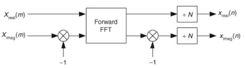
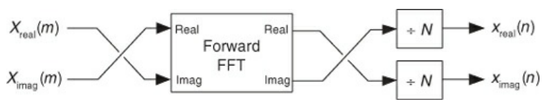
- The first method conjugates signal, does the FFT, then conjugates again
- The second swaps the real and imaginary components, does the FFT, then swaps the output
- You can easily prove the above two are equivalent to the inverse FFT by chugging through the algebra
Folded FIRs
- If an FIR filter has symmetric coefficients, then you can reduce the number of multiplications by roughly half
- Simply add up the signals which share the same coefficient (so if you have 5 taps, signal 0 adds to signal 4, signal 1 adds to signal 3 etc.), then multiply by the coefficient
Reducing ADC Quantization Noise
- Option 1: simply increase the sampling rate
- The noise scales like the inverse sampling frequency
- Option 2: dither. This means add some noise to the analog signal prior to discretizing
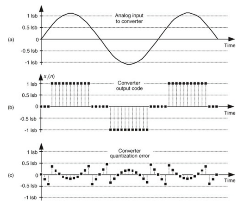
- This seems like a stupid idea, but it’s apparently not
- Take for instance the case of clipping. If an analog signal goes outside the range of the ADC, then values will get pegged to the maximum/minimum outputs of the ADC
- This clipping creates artificial spectral harmonics
- Another way of saying this is that clipping causes the quantization noise to become coherent with the signal
- If you dither an analog signal, then the quantization noise becomes less coherent, which means that these stray spectra harmonics are dampened
- Your noise floor increases as as result, but the SNR also increases due to the elimination of the stray harmonics
- This clipping creates artificial spectral harmonics
- You can use dithering for
- low amplitude analog signals
- highly periodic analog signals
- slowly varying analog signals
ADC Tests
Coherence Sampling
- Imagine that you feed a single sine wave of unity amplitude into an ADC. This will span the full range ADC and let you characterize the response of the ADC via an FFT
- there is spectral leakage that needs to be mitigated for this to work. the main trick is to have the ADC sampling rate be coherent with the signal frequency. This means that $f_{sample} = \frac{mf_{sig}}{n}$
- The choice of m and n matter. People have found that if you make m a odd prime number help minimize the redundant output codes of the ADC and make the quantization more random (desirable in this case)
- The FFT amplitude gets boosted by a factor of $10 * log_{10}(\frac{64}{2})$, so the actual SNR of the signal is smaller than the FFT would suggest
SINAD (Signal to Noise and Distortion)
- Also called SNDR
- To get a better indicator of the SNR, calcualate the SINAD
- Do the N Point FFT of the sequence and discard the negative frequencies
- Compute the total signal spectral power (re: summ the square of the bins with signal in them)
- sum the total noise-only spectral power
- Calculate $SINAD = 10* log_{10}(\frac{P_{sig}}{P_{noise}})$
Dynamic Range Testing
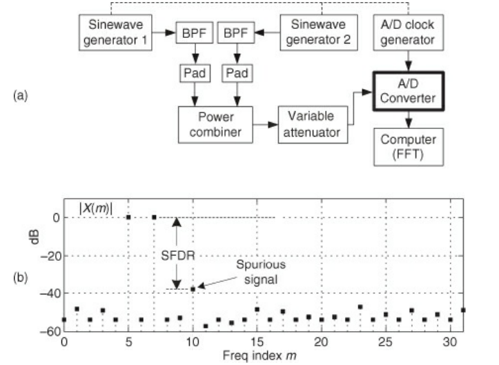
- To test the dynamic range, feed two equal amplitude analog sinewaves into an ADC
- Increase the amplitudes until you get some spurious spectral component which rises above the noise floor
- Define the SFDR as the dB difference between the high level signal spectral magnitude sample and the spurious spectral signal
Missing Codes
- Occasionally, ADCs will be incapable of producing a specific binary word (re: a code). so for an 8-bit ADC, it could happen that the number 33 is never output
- Just histogram all of the output values. Any missing codes will show up as 0 bins
Time Domain Convolution as FFT
- In some cases, doing a time domain convolution in frequency space is faster than the FIR implementation
- Simply break up the signal into chunks (with a power of 2 size per chunk, zero padding as needed), FFT each of them, multiply in frequency space, then inverse FFT
Sharpening FIR Filters
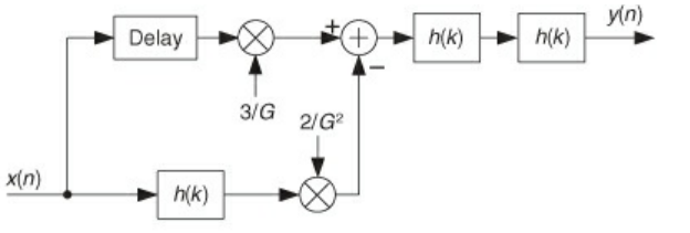
- Suppose that you want to improve the stopband attentuation of a FIR filter, but you can’t change its coefficients
- You could double up the filter (re: make a copy, then run it after the first), but this also increases the passband ripple
- Alternatively, you can do the above to keep the stopband attenuation, but reduce the ripple power
- G denotes the desired gain of the signal
- The Delay block is a consists ofo $\frac{N-1}{2}$ delays where N is the number of samples
- The x2 and x3 can be implemented via left shift by 1, and left shift by 1 added to original signal
- I don’t know why this works since the book doesn’t give a derivation
Goertzel Algorithm
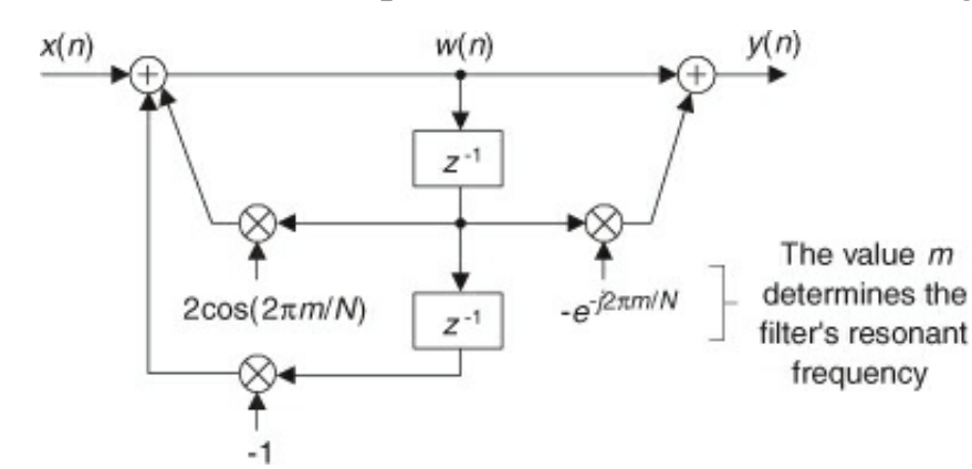
- Say you want to detect if a single frequency is in a signal. You could do an FFT, then check if the bin you want is above some threshold. But that requires computing the full FFT
- Goertzel’s algorithm lets you only compute a subset of the bins of a DFT
- As pictured above, Goertzel has two feedback coefficients, and one feedforward one
- The time domain difference equations are:
- $w(n) = 2\cos(\frac{2\pi m}{N}) w(n-1) -w(n-2) + x(n)$
- $y(n) = w(n)-exp(-i \frac{2 \pi m}{N}) w(n-1)$
- The time domain difference equations are:
- As pictured above, Goertzel has two feedback coefficients, and one feedforward one
- The transfer function of the IIR filter is as follows:
- $\frac{Y(z)}{X(z)} = \frac{1-exp(-i \frac{2\pi m }{N})z^{-1}}{1- 2 \cos (\frac{2\pi m }{N}) z^{-1}+z^{-2}}$
- There is both a pole and zero at $exp(-i\frac{2\pi m}{N})$ (plus a conjugate pole which doesn’t cancel out)
- The frequency response is to become sharply peaked around the m frequency bin
- The one surviving pole is on the unit circle, which might cause stability problems
- Luckily, the algorithm resets w(n-1) and w(n-2) for after each block, preventing the filter from running for too long and hitting instability
- The advantages of Goertzel’s algorithm over the FFT:
- N doesn’t need to be a power of 2
- The resonant frequency can by anything between 0 and $f_{s}$ Hz
- The number of coefficients is much smaller
- You don’t need to wait for the entire block of data to come in before starting the FFT
- You can implement M copies of Goertzel for multi-frequency detection and it will still be more efficient than an FFT if $M < log_{2}(N) $
- When doing Goertzel, you only retain every Nth sample. This causes the frequency response to become a sinc function
Sliding DFT
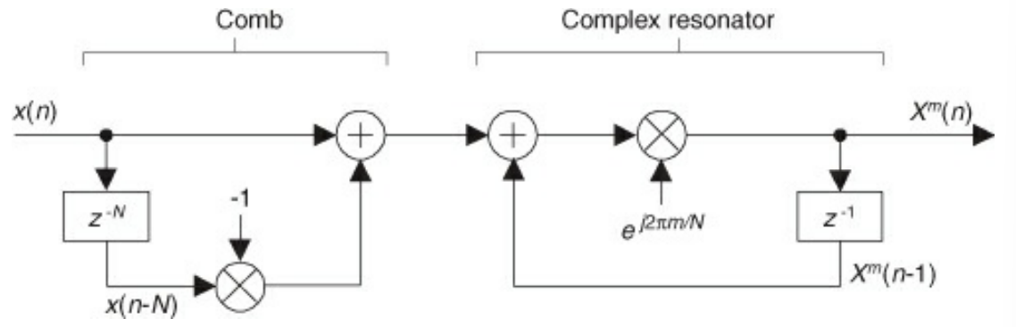
- Goertzel’s algorithm compute a single complex DFT bin for every N input samples
- The Sliding window algorithm lets you compute a DFT bin on a sample-by-sample basis
- You can evaluate the DFT for a single m bin:
- $X^{m}(q+1) = \Sigma_{n=0}^{N-1} x(n+q+1) exp(-i \frac{2\pi mn}{N})$
- The moniker “sliding” comes from the fact that the x(n) values used to compute $X^{q}$ gets shifted over by 1 every time step
- You can do some index juggling to tease out a recurence relationship for $X^{m}$
- $X^{m}(q+1) = exp(i \frac{2\pi m}{N})(X^{m}(q)+x(q+N)-x(q)$
- This version appears to look ahead at the future. That’s impossible. You can index on n instead of q to get: $X^{m}(q+1) = exp(i \frac{2\pi m}{N})(X^{m}(n-1)+x(n)-x(n-N)$
- $X^{m}(q+1) = exp(i \frac{2\pi m}{N})(X^{m}(q)+x(q+N)-x(q)$
- This have a pole on the unit circle, which can result in stability issues
- This can be mitigated by multiplying by $-r^{N}$ instead of -1 where r<1
Zoom DFT
- Instead of taking the FFT over a large number of samples, you get get a better frequency resolution around some region centered at $f_{c}$ with the above scheme
- There is an inflection point where using a Zoom FFT is more advantageous compared to just using a higher resolution FFT
Fast Arctangent
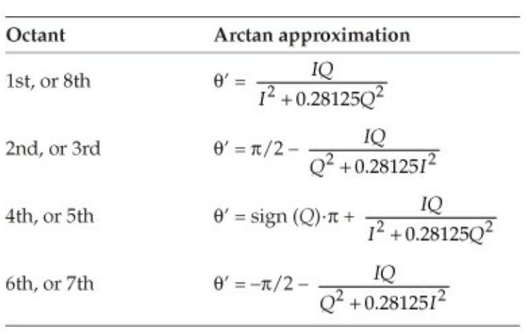
- Sometimes, you need to compute the phase of a quadrature signal
- let x = I+iQ. Can use above to do a dirty arctan caclutation
- depends on the Octant you’re in (start at real axis, increase index in a counter-clockwise manner)
Frequency Demodulation
- Tying into the above, we can calculate the instantaneous frequency of a signal by:
- converting it to a quadrature signal ( $ x=X+iY = A \exp(i\theta) = A \exp(2\pi f t i)$)
- calculating the phase ($ \theta = tan^{-1}(\frac{Y}{X})$)
- differentiating the phase w.r.t. time ($\Delta \theta$)
- use $f = f_{s}\frac{\Delta\theta}{2 \pi}$ to map the change in phase to a frequency
- If you want to avoid doing the costly arctan calculation, just take the derivative of $\arctan(\frac{Y}{X})$ with respect to time
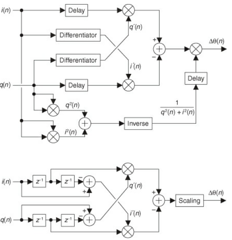
- Doing that yields the top schematic
- If you know the magnitude of your signal is constant (re purely frequency modulation), then the denominator can be dropped and you can use a basic central difference scheme for differentiation
- This is the bottom schematic
DC Removal
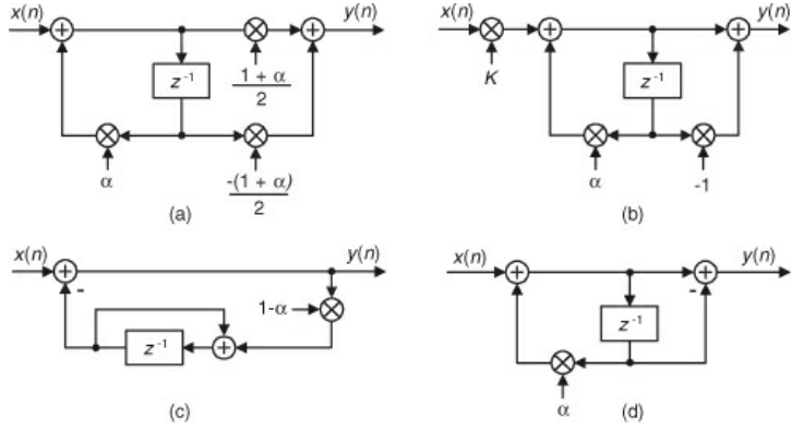
- Simplest way is compute the average of a block of length N, then subtract this from the each original sample
- This is not real time
- The IIR Filters above do real time DC removal
- They are all equivalent
- Their response functions are $H(z) = \frac{1-z^{-1}}{1-\alpha z^{-1}}$
- There is a zero at z=1, and a pole at $\alpha$
- The zero means that there is infinite attenuation at DC
- As $\alpha$ approaches 1, then the attenuation around the DC point gets sharper
- The phase experiences a jump discontinuity at DC and tappers off away from DC
Efficient Polynomial Evaluation
Horner’s Rule
- A standard kth order polynomial looks like:
- $f_{k}(x) = \Sigma_{0}^{k} c_{k}x^{k}
- You can massage the above to be written in terms of FMA (fused multiplication and addition), which is dedicated hardware circuit on some devices
- For specificity, look at the cubic. We have $c_{3}x^{3}+c_{2}x^{2}+c_{1}x^{1}+c_{0} = x(x(c_{3}x + c_{2}) + c_{1}) + c_{0}$
- The above is easily generalizable, and each group can be performed with FMA
- With fixed point, large left and right shifts can cause overflow
- A similar trick applies to this case, but swap multiplication for shifting
Estrin’s Method
- Horner’s Rule is inherently serial. You can parallelize it via writing the polynomials as nested expressions with a base rule of $ax^{q}+b$
- This maps well onto parallel MAC operations found in most modern CPUs
High Order FIR Filters
- How do you create a high-order FIR filter when your DSP software using Parks-McClellan refuses to converge
- In brief, you make a lower order FIR filter whose response is a crude approximation of your desired response, then you zero pad the frequency responese and recalculate the new coefficients
- In detail:
- Define a target number of taps to be M*N
- Set the number of taps in the lower order FIR filter (hence forth the prototype filter) to be N
- After calculating the coefficients for the prototype, perform an N-point DFT to get frequency response of the prototype
- Insert M-1 zero-valued samples just before the $\frac{N}{2}$ sample of the frequency response to get the new frequency response
- Calculate the inverse DSP to get the new interpolated FIR coefficients
- Take the real part to deal with finite precision issues
- Multiply the coefficients by M to compensate for the 1/M amplitude loss
- Test the interpolated coefficients (re: compare the FFT of the interpolated coefficients to the FFT of a massively zero padded version of the interpolated coefficients)
Automatic Gain Control (AGC)
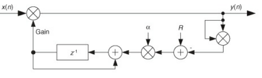
- The simple linear AGC circuit compares subtracts off the signals output power from some desired reference power, then feeds back this difference with some scaling factor $\alpha$
- There is some lag time before the signal returns to the constant power output. This lag/attack time is input dependent
- This lack of control over the attack time leads nicely to a logarithmic AGC design
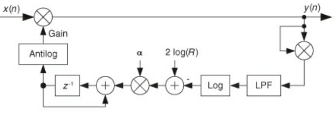
- The logarithmic AGC gives you more control over the attack time of the filter
- The low pass filter helps suppress rapid changes in the input
- The logarithmic design also has more dynamic range in comparision to the linear one
Quadrature Osscillator
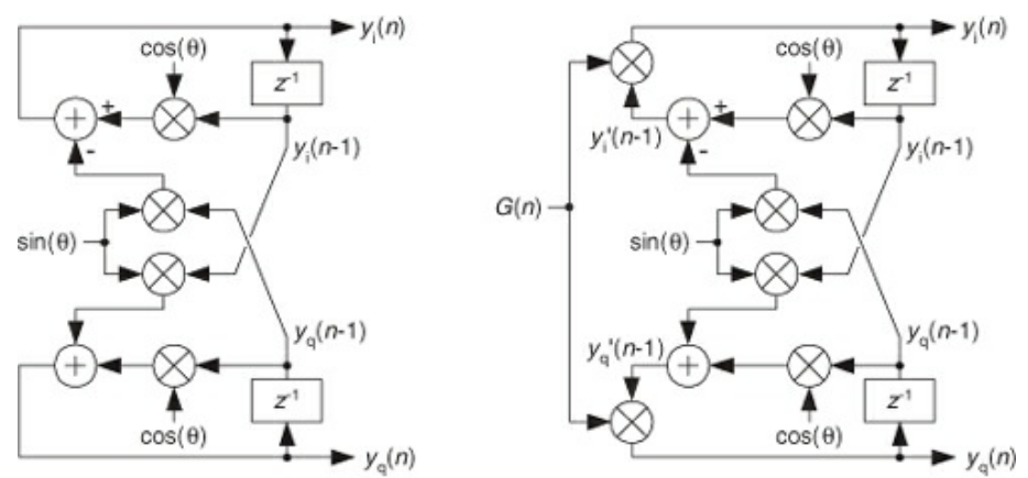
- The difference equation is given as
- $y_{r}(n) = y_{r}(n-1)\cos\theta - y_{i}(n-1) \sin \theta$
- $y_{i}(n) = y_{r}(n-1)\sin\theta + q_{i}(n-1) \cos\theta$
- This is just multiplying the previous input by $e^{i\theta}$
- One big problem is that the input can grow/decay out of control. introduce AGC into the mix
Faster Variance
- The unbiased variance can be re-written as $\sigma_{ub} = \frac{\Sigma_{n=1}^{N} (x(n)^{2}) - Nx_{avg}^{2}}{N-1}$
- This introduces two additional multiplications at the expense of N fewer additions
- In the standard formula, we need to retain the all of the N samples in order to computer the average. With this set up, we don’t need to do that
Signal Transition Detection
- Suppose that you need to detect a transition in an input which spans many samples. A standard digital differentiator would have the memory to accomudate that.
- We can use the so called “time-domain slope filtering”, which is a FIR filter with the following coefficients:
- $C_{k} = -\frac{12k-6(N-1)}{N^{3}-N}$ where N is any integer
- The affect of the above is to create a linear ramp in coefficient value
- This approach is more robust against high noise levels in comparision to a standard digital filter