An introduction to databases.
- Logistics
- Intro
- Database Design
- ER Model
- SQL (Structed Query Language)
- Object-relational Databases
- Physical Storage
- Indexing
- Transactions
- Query Processing
Logistics
-
Location: Havermeyer 325
-
Time: 2:40-4:00
-
Grading Scheme
- Homework: 0% (but should do all 4 of them anyways)
- Project: 30%
- Midterm: 20% (March 6th)
- Final: 50%
Intro
- Database management system (DBMS) used to organize data in a way that is convenient (easy to read and write to) and efficient (fast to read and write)
- Databases solve a number of problems with storing data
- Data redundancy and inconsistency
- Data might be unnecessarily repeated, or repeated copies might not agree with each other
- Difficulty in accessing data
- Database systems allows people to more easily retrieve data
- Data isolation
- Certain applications need access to only some data, not all of it
- Integrity problems
- Some quantities must have constraints on them (for instance, the balance amount of a department’s budget must be greater than 0)
- Atomicity
- An atomic operation means an all or nothing operation
- This means that either the operation happens completely, or it does not happen
- An atomic operation cannot create some intermediate state
- For databases, this is important, since some updates logically must be atomic (like wire transfers)
- An atomic operation means an all or nothing operation
- Concurrency
- Since many users can access database at same time, need to make sure that database always remains valid
- Security
- Not all users need access to all data
- Data redundancy and inconsistency
- Instance: the collection of information stored in a database at a given time
- Schema: The overall design of the database
- ie. The Columns of all of your tables
- Can think of two primary modes in which databases are used
- online transaction processing: you have a large number of users simultaneously accessing the database, where each user makes a small number of queries consistently
- data analytics: you process a large amount of data to draw conclusions
Data Models
-
ER Model
- You have entities and relationships
-
Relational Model
- A collection of tables to represent both the data and the relation amongst the data
-
Entity-Relationship Model
-
Semi-structured
- Think JSON or XML
- Individual data items of the same type may have a different set of attributes
Database Design
Phases
-
Requirements gathering
- The hardest part. Getting people to tell you unambiguously tell you what they want
- What data the users want to store, and how they want to interact with that data
- Avoid conflicting requirements
-
Schema generation
- Translating text description of data to constraints, entities, relationships
Bad Design
- Make sure that when designing stuff, you don’t do the following:
- Redundancy
- Information appear in exactly one place
- Incomplete
- The ER diagram does not properly model reality/ makes certain tasks difficult
- Redundancy
ER Model
-
Entity: a thing in the real world that is distinguishable from other things
- Really generic/vague
- Like to think about entities as something important to your domain application that you want to store info about
- So if you are storing data on NFL games, “Teams” would be an entity, since you want to have info about each team
- Each entity has some properties associated with it
- Each entity must have some set of properties that uniquely identify the entity from other instances of the entity
-
Entity Set: a set of entities of the same type that share the same properties or attributes
- Extension: the actual collection of entities belonging to an entity set. Used when talking about entity sets in abstract; extension makes concrete entity sets
- Entity sets do not need to be disjoint (ie. different types of entities can exist in an entity set)
-
Attributes:
- descriptive properties possessed by each member in an entity set
- Each entity many have it’s own value for each attribute
- Typically, there is some ID attribute to uniquely identify the entity
-
Relationship: An associate among several entities
- So if Player and Team are entities, can think of the relationship between them as “A Player must be in a Team”
- Relationships can have attributes associated with them (called descriptive attributes)
- So if a Student Takes a Course, then you could assign a Grade attribute to the Takes relationship
-
Relationship Set: A set of relationships of the same type
-
Relationship Instance: An association between named entities
- So a concrete example of a particular relationship
-
Weak Entities:
- An entity whose existence is contingent on the existence of another entity
Drawing ER Diagrams
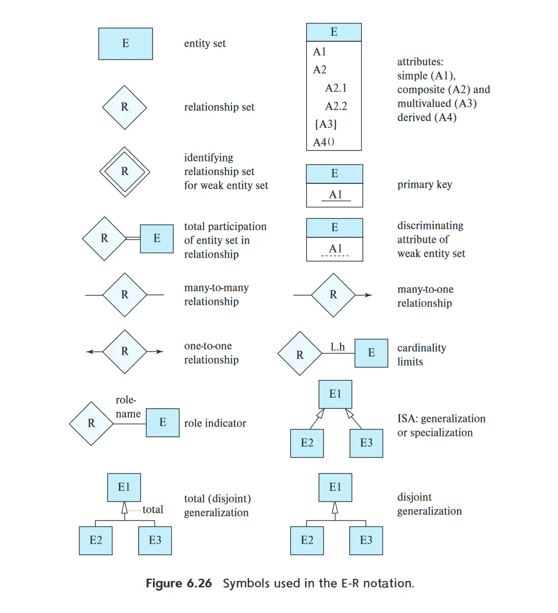
- An entity/ entity set is represented by a rectangle, subdivided into two parts
- The top portion names the entity set
- The bottom portion contains the names of all the attributes of the entity set
- The primary key/attribute of the entity should be underlined
- Relationships are drawn as diamonds, with different types of lines connecting its associated entites together
- Attributes of a relationship are modelled as an undivided rectangle
- The undivided rectangle is linked with a dashed line to the relationship
- For a binary relationship, the lines from the diamond can have arrows on them which point to the associated entity, Their meaning depends on what the over line is annotated as
- One to one: both lines have arrows
- One to many/ many to one: the One attribute has the arrow
- Many to many: no arrows on either line
- Can model Cardinality (say, that there must be at least 2 birth parents to a child) with numbers near the links
- Attributes of a relationship are modelled as an undivided rectangle
- Weak Entities are drawn as double rectangle. The discriminator (ie. the additional attributes that distinguish the weak entity from others) is underlined with a dashed line
- The relationship associating the weak entity to the strong entity is a double diamond
- Can use double lines to denote that a relationship is total
- This means that the weak entity must be relation via the relationship to the strong entity
SQL (Structed Query Language)
-
Physical manifestation of E/R models and/or relational databases
-
Basic types
Type Description char(n) a fixed length character string varchar(n) a variable length character string with at most n characters. Prefer this over char nvarchar(n) a variable length character string of Unicode characters. Use for multilingual strings int integer as defined by machine smallint small integer (like a char in C) numeric(p,d) A fixed point number with user specified precision. p digits long, with d digits to the right of the decimal place real machine dependent floating numbers float(n) a floating-point number with precision of at least n digits -
All types can include a special value called null
- Can interpret as the absence of a value from the database
SQL Schema
-
To define a Schema (ie. a table name and it’s columns), we use the create_table command. The format is as follows:
- create table TABLE_NAME (
$A_{1} D_{1}$,
$A_{2} D_{2}$,
…
$A_{n} D_{n}$,
primary key ($A_{i}$) )
- In words, you are creating some table TABLE_NAME with some N attributes A of datatypes D. THe primary key is some attribute $A_{i}$
- You can also have foreign key($A_{i}$) and not null($A_{i}$) to denote a foreign key and that a value cannot be null
-
You can remove a table from a database with the following syntax:
DROP TABLE <table_name> -
You can delete all the rows from a table with
DELETE FROM <table>command -
You can add to a table with the alter table command:
alter table r add A D- r is the table name
- A is the new attribute
- D is the datatype of the attribute
-
Some (but not all) flavors of sql allow you to drop specific attributes:
alter table r drop A
SQL Query Anatomy
- A basic SQL query consists of 3 clauses: select, from, where
- More generally, one can think of an SQL query as follows:
- Generate a Cartesian product of relations listed in the FROM clause
- Apply the predicates specified in the WHERE clause on the result of Step 1
- For each tuple in the result of Step 2, output the attributes/ expression results specified in the select clause
- All SQL queries end in a semicolon (;)
SELECT and FROM
- Select allows you to pull out specific attributes from a table, while FROM specifies what table you want to apply an operator to
- Ex:
SELECT dept_name FROM instructorwill pull the department name of each instructor - You can specify multiple attributes to pull (
SELECT dep_name, salary FROM instructor), or you can use a wildcard to get all the attributes (SELECT * FROM instructor) - You can apply additional keywords to attributes to refine your search. For instance, the
distinctkeyword enables one to only take all the unique rows for a given query- The opposite keyword
allforces SQL to include all duplicates. This is the default behavior though
- The opposite keyword
- You can do arithmetic operators if the attribute type is ammenable to said operator. For instance:
SELECT salary*1.1 FROM instructor- Some date types also allow arithmetic operations
- Ex:
- You can select from multiple tables, but if two tables share the same attribute name, you must specify which table you want to pull from. This applies throughout the sql query
- Ex
select name, instructor.dept name, building from instructor, department where instructor.dept name= department.dept name; - If you want to get all the attributes of a specific table, you can use the syntax:
table.*
- Ex
WHERE
- the WHERE clause allows filtering if a query so that entries match certain constraints.
- For instance:
SELECT name FROM instructor WHERE salary > 70000- You can chain multiple constraints together with logical operations like
and,or, andnot. Ex:SELECT name FROM instructor WHERE salary > 70000 AND salary < 100000A more concise notation for ANDing constraints is the tuple notation:select name, course id from instructor, teaches where (instructor.ID, dept name) = (teaches.ID, 'Biology');
- You can chain multiple constraints together with logical operations like
- For instance:
AS keyword
- When doing multitable selections, you can disambiguate which table you are selecting from via the
askeyword. This is called a table alias- Ex:
select T.name, S.course id from instructor as T, teaches as S where T.ID= S.ID; - This is useful when comparing a relationship to itself:
select distinct T.name from instructor as T, instructor as S where T.salary > S.salary and S.dept name = 'Biology';- Can’t use instructor.salary since it is ambiguous wheather you are referring to T or S
- Ex:
String Operations
- SQL strings are specified by enclosing them in single quotes
- You can escape single quotes by using two single quotes instead of 1
- Ex: It’s right becomes ‘It’’s right’
- The SQL standard demands case-sensitivity when doing string comparisons. However, not all implementations strictly enforce this
- You can escape single quotes by using two single quotes instead of 1
- You can do certain string specific operations on the resulting string from a query
- ‘||’ concatenates strings
- upper(s) and lower(s) converts strings to upper and lower respectively
- trim(s) removes trailing spaces
LIKE
- You can do pattern matching with the
LIKEkeyword- Syntax is like:
SELECT A FROM T WHERE P like 'pattern'; - Pattern are case-sensitive
- There are some special characters for pattern matching
%means that you match any substring_means that you match any single character- If you want to search or a special character, utilize an escape character (typically a ‘')
- If you want to search for mismatches instead, use the
NOT LIKEoperator
- Syntax is like:
ORDER BY
- You can control how the output rows are displayed via via the
ORDER BYkeyword- Can use
descto sort in descending order, andascfor ascending - Can order by on multiple attributes (useful for breaking ties)
- Ex:
SELECT * FROM instructor ORDER BY salary desc, name asc;
- Can use
Set Operations
- Can think of the result of all SQL queries as being a part of a relational algebra. Hence, we can do set operations on them
UNION
- When you want to take the union of two SQL queries (ie. see results that appear in either table1 or table2), use
UNIONkeyword. This automatically remove all the duplicates which appear in both tables- Syntax:
(table1) UNION (table2)- The parentheses are optional
- If you want to preserve duplicates, use the syntax
UNION ALLinstead
- Syntax:
INTERSECT
- When you want to see results that appear in both table1 and table2, use
INTERSECT- Syntax:
(table1) INTERSECT (table2) - Same caveat as union: removes duplicates implicitly. If you want to preserve dups, tack on ALL
- Syntax:
EXPECT
- If you want to find tuples in table1 but not table2, utilize the
exceptkeyword- This outputs all tuples found in the first table that do not occur in the second table
- All duplicates are eliminates prior to performing the set difference
- Same all keyword caveat holds
Null Values
- If you do arithmetic operators on a NULL value, the result is always NULL
- If you do logical operators on NULL values, it is ambiguous whether the statement should evaluate to TRUE or FALSE
- SQL circumvents this problem by introducing a third state called UNKNOWN
- If the predicate of a WHERE clause returns FALSE or UNKNOWN, that those rows are not added to the output
- Below is a table listing how the boolean operators interact with this new third state
| OPERATOR | LEFT OPERAND | RIGHT OPERAND | RESULT |
|---|---|---|---|
| AND | TRUE | UNKNOWN | UNKNOWN |
| AND | FALSE | UNKNOWN | UNKNOWN |
| AND | UNKNOWN | UNKNOWN | UNKNOWN |
| OR | TRUE | UNKNOWN | TRUE |
| OR | FALSE | UNKNOWN | FALSE |
| OR | UNKNOWN | UNKNOWN | UNKNOWN |
| NOT | N/A | UNKNOWN | UNKNOWN |
- You can test for UNKNOWN results via
IS UNKNOWNandIS NOT UNKNOWNkeywords - You can test for NULL results via
IS NULLandIS NOT NULLkeywords
Aggregation
- Aggregate functions take a collection of values and returns a single value
- SQL comes with 5 in build aggregate functions: AVG, MIN, MAX, SUM, COUNT
- SUM and AVG must be a collection of numbers
- Ex:
select avg (salary) from instructor where dept name = 'Comp. Sci.'; - By default, no duplicates are included. If you want to exclude duplicates (say, you are counting unique IDs), prepend the
DISTINCTkeyword to the attribute being aggregated on - You can use wildcard * in order to just pass all the rows into an aggregate function (useful for COUNT)
- When dealing with NULL values, the default for most aggregate functions is to ignore the NULL rows
- COUNT does NOT do this. COUNT includes the NULL
- If all values passed to an aggregate are NULL, then the return value is NULL
- COUNT just returns 0 in this case
GROUP BY
- You can use
GROUP BYkeyword to perform aggregation on a group by group basis instead of all the rows together as a collective- Ex:
select dept name, avg (salary) as avg salary from instructor group by dept name;- This query finds the average salary in each department
- It’s important that the all attributes NOT part of the aggregator function are included in the GROUP BY clause. Otherwise, the query is malformed
- Ex:
HAVING
- If you want to perform validity constraints at a group level instead of a tuple level, you can use the
HAVINGkeyword- Ex:
select dept name, avg (salary) as avg salary from instructor group by dept name having avg (salary) > 42000;- This selects all deptments whose average salary is greater than $42000
- Ex:
Nested Subqueries
- You can nest one SQL expression inside another one in either the WHERE or the FROM clause
- In either case, wrap the nested query in parentheses
Subquery tests for WHERE
- When doing it inside the WHERE clause, you can use the
INandNOT INkeywordsselect distinct course id from section where semester = 'Fall' and year= 2017 and course id in (select course id from section where semester = 'Spring' and year= 2018);- The distinct is necessary to remove duplicates
- You can use a table alias from the outer query in the inner query
- Sometimes, a subquery might return nothing. You can use the
EXISTS(<sub_query>)operator instead of the IN keyword to check if the query returned anything - Additionally, sometimes you want to check if all the subquery results are unique. You can use the
UNIQUE(<sub_query>)operator - You can negate both of these with the NOT keyword
Subquery test for FROM
- When doing a nested subquery inside FROM clause, you don’t need additional keywords according to the SQL standard. Just wrap in parentheses
- If you are using PostgreSQL, you need to table alias the statement with an AS keyword
DELETE, INSERT, UPDATE
DELETE
- The syntax of delete is:
DELETE FROM table WHERE P - You can only operate on one predicate at a time
- That predicate can be a complex nexted subquery
INSERT
- Syntax is
INSERT INTO table(attr1,attr2) VALUES (val1, val2) - You don’t need to specify all the attributes of a table. SQL will fill those in with NULLs, assuming no NOT NULL constraints
- You can also pass a SELECT statement into an INSERT statement
UPDATE
- Syntax is:
UPDATE table SET attr_name=new_value- You can reference the attribute name in the updated value (ie. salary=salary*1.05 to present a 5% pay raise)
- You can apply WHERE operations after the SET clause
JOINS
Joins are an alternate way of joining two relationships together
Natural/Inner Joins
- Natural joins combines two relations into a single relation. In doing so, it only considers tuples where both the LHS and RHS share a common attribute
- In general:
select A1, A2, …, An from r1 natural join r2 natural join ... natural join rm where P; - You can specify which columns to join on with the
ONkeyword select * from student join takes on student.ID = takes.ID;
- In general:
Outer Joins
- Let’s say that you want to join two tables, but want to include values not found in both tables
- Outer Joins let you do this, by filling in missing values with NULLs
- There are 3 flavors: left, right, and full
- left outer joins preserves tuples only in the left operand of the join
- right outer joins do the same, but on the right
- full preserves tuples in both relations (ie. the union of the left and right outer joins)
Views
- Let’s say that you want to restrict certain types of users to only be able to view certain attributes of a table. You can use views
Syntax: CREATE VIEW v as <query_expression>- Can think of views as precompiled queries that get run on demand
- You can make views of view
- You can’t modify a relation through a view (normally, caveats are complicated and not necessary for this class)
Integrity Constraints
- Not Null: specifies that NULL is not allowed for this attribute. Syntax is
attr NOT NULL - Unique: syntax is
UNIQUE(A1,A2,...An)- States that no tuple can have be equal on the listed attributes
- Attributes are permitted to be null unless specified otherwise
- Primary Key(s): all primary keys are required to be non-null and unique. Syntax is
primary key (attr)- Most SQL flavors provide someway of auto-generating primary keys. However, it is implementation dependent
- Foreign Key: a constraint that requires that a particular attribute appears in another table. Syntax is
foreign key (attr) references foreign_table(foreign_attr)- Can be null unless explicitly NOT NULL constrained
- Can append
on delete cascadeoron update cascadeafter foreign table to have foreign keys get deleted/updated in foreign table is value in current table changes
- Check: syntax is
check(P)where P is some arbitrary predicate- Practically, what P can be is limited to relatively simple things
- If P evaluates to unknown, then the check clause is NOT violated
- You can give names to a constraint with the
constraintkeywordsalary numeric(8,2), constraint minsalary check (salary > 29000),- This allows one to drop a particular constraint more easily
- All of the above constraints can be specified as
deferred. This means that the constraint will be checked at the end of a transaction, rather than in the intermediate steps - You can also provide user-defined types in order
create type Dollars as numeric(12,2) final;- User defined types wrapping the same built in type are NOT equivalent. You need to cast them first
Authorization
- The top level hierarchy of a database is called the catalog
- Each catalog can have multiple different schema assigned to it
- Each schema can have it’s own tables associated with it/shared with other schema
- All SQL queries operate within the context of a schema
- Schemas are typically created automatically with new user accounts, in either a default catalog, or some special catalog for new users
- Each catalog can have multiple different schema assigned to it
- The reason for all of the gobbledygook above is so that each user/application only has access to the things that they need access to. This allows multiple users/applications to access the same data without stepping on each other’s toes
Privileges
- There are 5 privileges that one can bestow upon users: Read, Insert, Update, Delete, and References
- Privileges can be given/taken away with the
grantandrevoke- Grant syntax:
grant <privilege list> on <relation name or view name> to <user/role list>;- Can use
all privilegesto grant user all 4 privileges - Can omit
onclause - For update and insert, one can specify which values can be modified with a (attr_name) after the privilege
- Can use
- Revoke syntax:
revoke <privilege list> on <relation name or view name> from <user/role list>;
- Grant syntax:
- You can allow users to pass on privileges by appending the
with grant optioncommand to the end of a grant statement- Under normal circumstances, removing privileges from a user also removes any privileges down the chain. you can prevent this behavior by appending
restrictto the end of the remove statement
- Under normal circumstances, removing privileges from a user also removes any privileges down the chain. you can prevent this behavior by appending
Roles
- Instead of granting each user individually all the permissions needed, you can define a role, grant each role the necessary permissions, and then grant each user particular role(s)
- Roles can inherit from each other
- Ex:
grant instructor to dean;Gives all the privileges of instructors to a dean
- Ex:
- Creating a view to some data does not let you escape your privileges. Any privileges (or lack thereof) gets applied to the view
Object-relational Databases
Complex Types
- Some systems require more flexible schema than that of standard SQL. For instance, web applications
- Some database systems allow a wide column representation, which means each tuple can have a different set of attributes
- A more restricted form of this is that each tuple shared a large number of attributes, but each tuple nulls out the unused attributes
- called sparse column
- A more restricted form of this is that each tuple shared a large number of attributes, but each tuple nulls out the unused attributes
- Some databases allow sets/multisets/arrays as attribute values
- For instance, in PostGre, using
integer[]denotes an integer array of unspecified length
- For instance, in PostGre, using
- Yet more allow you to store key-value maps (ie. hash tables)
- put(key,value) writes to map
- get(key) retrieves associated value
- delete(key) removes key-value pair from map
- There exist serialization formats which allow data representations which allow values to have complex internal structures without adhering to a fixed schema
- The most prolific are JSON (JavaScript Object Notation) and XML (Extensible Markup Language)
User Defined Types
- Users can defines their own custom types in most SQL flavors
- For instance, if you want to create a Person:
create type Person
(ID varchar(20) primary key,
name varchar(20),
address varchar(20))
ref from(ID);
create table people of Person;
- You can insert a custom type into a database via:
insert into people (ID, name, address) values
('12345', 'Srinivasan', '23 Coyote Run');
Inheritance
- You can inherit from previously defined types/tables, and add more attributes to the derived type
create type Teacher under Person
(salary integer);
- You can use an ORM (Object-relational mapping) system to allow you to bind types/tables directly to language specific objects (SQLAlchemy is a good example for Python)
Textual Data
- For many applications, you need to do some sort of textual lookup in the database and extract the relavent results
- This is what a web browser is at it’s core
- Let t be the term you want to look for and d be some document. You can define a basic term frequency metric to denote how relavent a document is to a term
- $TF(d,t) = log(1+\frac{n(d,t)}{n(d)})$
- $n(d,t)$ is the number of occurances of term t in document d
- $n(d)$ is the total number of terms in the document
- A query Q consists of multiple terms t. Naively, one can sum the relevancy of all the TF terms to get an overall document relevancy
- The above method can be augmented via a weighting scheme to account for rarer words
- $r(d,Q) = \Sigma_{t} TF(d,t) * \frac{1}{n(t)}$
- Some words, like a, and, or and so on don’t contain much useful information due to their high frequency, hence most algorithms just discard these words when calculating relevancy
Big Data
- The need to deal with huge amount of data requires large scale parallelization of data storage and processing
- Distributed file systems try and fulfill this requirement
- By sharding or partitioning records across multiple systems, databases can split the load of accessing files across multiple systems
- A single file (if it’s very large) can be split up and stored across multiple machines, at which point, you can parallelize the file reading for increased access speeds
- You can also store multiple copies of a file across many machine to increase redundancy and reduce the chance of losing a file
- By sharding or partitioning records across multiple systems, databases can split the load of accessing files across multiple systems
Streaming Data
- Some situations require that queries need to be constantly be executed on data that arrives in a continuous fashion
- Normal database queries need access to all the records to even begin optimization, let along actually execute the query. You can’t do this with streams, since in theory, they can go on indefinitely
- One way to deal with this is via windows, which either contains tuples that appear within a certain time window, or just contained a finite number of tuples
- One can then in theory figure out when you have sufficient context to execute a query
- On can also have the result of queries dynamically update as more data comes in
Physical Storage
Types
- 5 main types of memory relevant to databases
- Cache: the fastest and most expensive types of memory
- Main memory: volatile memory (RAM) upon which machine instructions operate on. In theory, for small enough operations, you could store a database here. It would get lost on power loss though
- Flash: non-volatile memory. SSDs are the defacto storage medium of long term storage
- Utilizes a block interface, in which data is stored/retrieved in fixed size blocks (ex. 512 bytes to 8 kilobytes)
- Magnetic disk storage: This is more long term than Flash memory. It’s also the slower since you physically need to move a head to read and write from the disk
- Tapes: magnetic taps are sequential storage devices that are the most stable storage medium listed here, but take seconds to read from. Primarily used for archive purposes.
Interfaces
- SATA (Serial ATA) interface and Serial Attached SCSI (SAS) interface is how hard drives communicate with the rest of the computer
- Non-Volatile Memory Express (NVMe) interfaces is the logical standard developed to better support SSDs and is typically used with PCIe interfaces
- The above interfaces utilize cables to connect storage. You can also use high speed networking to connect the computer
- SAN (storage area network) allow a large number of disks to be connected to a large number of computers
- NAS (Network attached storage) is similar to SAN, but instead of the networked storage appearing as a single large disk, it provides a file system interface
Magnetic Disks
- Magnetic discs are rigid platters which are covered with a magnetic material. These disks are then rotated at high speeds (5400 to 10,000 RPM)
- The disk is logically divided into tracks from inside out, and then which are further subdivided into sectors. Sectors are the smallest quanta of storage that can be read/written to the disk
- There is a read-write head, which can change the magnetization of of a particular sector to store information
- Some performance metric of disks:
- Access time: the time needed to read or write to the disk
- seek time: the time needed to reposition the head to the correct sector
- rotational latency time: The time needed to wait for the disk to spin the correct sector into place below the head
- data transfer rate: the total throughput at which data can be retrieved from or stored to the disk
- I/O Operations per second (IOPS) is the number of random block accesses that can be satisfied by a disk in a second
- depends on access time, block size, data transfer rate etc.
- Mean Time to Failure (MTTF) the expected time that a disk can be expected to run
- Typical mean MTTF is around 1E6 hours (decades!!!)
- This is computed probabilistically, so that if you have 1000 disks, then one is almost certain to fail by 1000 hours (So they are kind of lying)
- Typical mean MTTF is around 1E6 hours (decades!!!)
Flash
- Build with NAND flash. Can only read a page of data at a time (typically 4096 bytes)
- Random access times on the order of microseconds
- Writing to a page is more complicated. You can write to an empty page in around 100 microseconds
- If you want to overwrite a page, you need to first erase the block and then write to the disk
- Erasing can only be done on a group of pages (erase block) and takes around 5 milliseconds
- Pages can only handle a certain amount of erasing before they no longer function
- Erasing can only be done on a group of pages (erase block) and takes around 5 milliseconds
- Logical pages get mapped to physical pages via a translation table. Hence, if a particular page fails, the SSD can fail over to some reserved clean pages
- SSDs endeavor to evenly distribute erase operations across physical blocks (process called wear leveling)
- The performance of SSDs are characterized as follows:
- The number of random block reads per second (4 kilobyte blocks)
- SSDs support parallel random requests
- the data transfer rate
- The number of random block writes per second
- The number of random block reads per second (4 kilobyte blocks)
RAID
- Redundant array of independent disks (RAID) is collection of disk organization techniques for performance/reliability reasons
- Disks fail all the time. To mitigate catastrophic data loss, one store multiple copies of the data
- The simplest (and most expensive) approach is called mirroring (or shadowing) where each disk has a backup disk. The logical disk has two physical disks. Each write gets to write to both disks, while each read only accesses the primary disk. In case of a failure of either disk, you don’t lose data and you have time to replace the failed disk
- To increase performance, one can strip the data across multiple drives. What this means practically is that you store each block of data in some defined sequence across multiple drives. You can then read back from multiple disks in parallel to reconstruct the original data
RAID Levels
- Mirroring is expensive. Most people use parity blocks. What this means is that for a given set of blocks, a parity block is computed via XORing all the bits of the each block together. If a block gets corrupted, it can be recovered by XORing the rest of the blocks with the parity bit to recover the data
- Hence, you need to update the parity block whenever you update the block group
- The schemes that are used to enforce this kind of redundancy are called RAID levels
- RAID 0 is no redundancy. Only data striping is utilized
- RAID 1 is the mirrored disk setup
- RAID 5 is block-interleaved distributed parity. A particular disk store the parity disks of the rest of the disks in a subsection
- RAID 6 is called the P_Q redundancy scheme. It utilizes different error correcting codes. The upshot is that you can more disk failures before data loss in exchange for large resources allocated to redundancy
- RAID can be implemented in either software or hardware. Software takes a long time to re-silver the disks if disk failure occurs
- RAID also does something called scrubbing, where during periods where the disks are idle, RAID checks for damaged/corrupted sectors and updates them
- Certain server hardware permits hot swapping, which allows disk replacement without turning off the power. Useful for 24/7 systems
Indexing
- In order to be able to access a tuple in a relationship, you need an index to allow you to quickly identify which block the data you are looking for belongs to.
- Two types: Ordered (sorted in some order. implemented as a B+ tree) and hash (hash map)
- Some considerations to consider when deciding on an implementation of indices
- Access Types: certain types might be stored more efficiently
- Access time: the time it takes to find a particular data item
- Insertion time: time need to insert a new item. Includes finding the correct place to insert, as well as updating index
- Deletion time: analogous to insertion, but delete record
- Space overhead: how much additional space does the index require
Ordered Indices
- Clustering index/ primary index: an index whose search key also defines the sequential order of the file
- Indices whose search key specifies an order different from the sequential order of the file are called nonclustering/secondary indices
- An index record consists of a search-key value and pointers to one or more record with that value
- Dense index record: an index entry appears for every search-key value in the file
- Sparse: an index entry appear for only some search-key values. You need to find the closest search-key to index missing -search-keys
- You run into the problem that your index doesn’t fit into RAM, which makes accessing it slowly. This can be solved by making an index for the index, which is smaller and can fit in RAM. This schema can be nested
- If you have multiple values in a search-key they follow lexicographic ordering
- For instance, $(a_{1},a_{2}) < (b_{1}, b_{2})$ is true if either $a_{1}<b_{1}$ or $a_{1} = b_{1}$ and $a_{2} < b_{2}$
B+ Tree
- A balance binary tree where every path frmo root to leaf is of the same length
- It’s different from a binary tree since each leaf node is augmented with a pointer to the next leaf node. This allows easy traversal of the leaves
- Node have restrictions on how much/how little data can be in them
- Every leaf node can hold up to n-1 values and must have $ceil((n-1)/2)$ values in it
- The non leaf nodes (internal nodes) may hold up to n pointers and must hold at least $ceil(n/2)$ pointers (These pointers point to the next node on the same height of the tree)
- The root node must hold at leas two pointers (unless the tree is only one node)
- With the above restrictions, the path length between a root and leaf is constant amongst all leaves due to pointers allowing shortcuts
- Keys should be unique can for uniqueness by addition primary key of relationship r to index if collision occurs
Hash Indices
- Bucket: a unit of storage that can store one or more records
- A hash function h is defined as a function from the set of all search-key values K to the set of all bucket addresses B
- If a collision occurs, and you can’t fit more data into a bucket, it’s called bucket overflow. You need to write the data to a new bucket that is linked to the first bucket
- Fixing the number of buckets on startup is called static hashing. To prevent bucket overflow, you could double the number of buckets, and then rebin the data when needed. This is slow. There are other schemes on how to do this more efficiently, called dynamic hashing
Transactions
- a transaction is a unit of program execution that must appear as a single, indivisible unit from the outside (this is called atomicity)
- Ex: Transferring funds between account
- To ensure atomicity holds, we need some way of rolling back changes if something fails. a log file typically stores the intermediate values, and if something goes wrong, it can undo all the actions done (ie. it aborts the transaction and rolls back). This prevents the database from being in a user-facing inconsistent state
- Care also needs to be taken that transactions don’t affect each other concurrent transactions until they are finished (called isolation)
- Assuming that data to disk never gets lost, we need to write information that will enable rollback to the disk, as well as the final database state
- You need some concurrency control system (locks) in order to prevent this from happening
- Or you could do it serially. But that doesn’t scale as well
- Assuming that data to disk never gets lost, we need to write information that will enable rollback to the disk, as well as the final database state
- Actions of transactions must persist across crashes (durability)
- The database state should maintain some invariant as defined by the transaction programmer (consistency)
- Collectively, these are called ACI properties
- If a transaction finishes without errors, it’s said to be committed. This places the database in a new consistent, persistent state
Scheduling
- Figuring out in what order to execute parallel transactions is called scheduling. This is a common problem in a lot of branches of computation (like operation systems)
- Not all schedules are serializable (ie. have the same result as performing all the transactions serially)
- There are four cases that need to be considered when two transactions are touching the same tuple Q
- I:Read, J:Read. Order doesn’t matter here
- I: Read, J: Write. If I comes before J, then the first transaction does not read the value of Q that is written by J. If J comes before I, then the first transaction does read the value written by J
- The above is symmetric for I: Write, J: Read
- I: Write, J: Write. Since both instructions are write, the ordering does not affect either the first or second transaction. The next read WILL be affected, since only the last write call is preserved
- To determine if a given schedule can be serialized, turn it into a precedence graph, which is a DAG consisting of vertices V and edges E
- V is the set of all transactions participating in the schedule
- E is the set of all transitions from $T_{i}$ to $T_{j}$ for which one of the following three conditions hold:
- $T_{i}$ executes write(Q) before $T_{j}$ executes read(Q)
- $T_{i}$ executes read(Q) before $T_{j}$ executes write(Q)
- $T_{i}$ executes write(Q) before $T_{j}$ executes write(Q)
- If there is a cycle in the precedence graph, then the schedule cannot be serialized
- This is called topological sorting
- What happens if you run a schedule, but the transaction fails? You need to be able to roll back this partial schedule
- Some schedules cannot be recovered from. For instance, if one transaction finishes and commits it changes halfway through another, and it running transaction fails, you can’t roll back since you have lost the previously committed state
- There are edge cases where a single transaction failure causes a series of transaction rollbacks (called cascading rollback)
- Ideally, want a cascadeless schedule, which is one where from each pair of transactions $T_{i}$ and $T_{j}$ such that $T_{j}$ reads a data item previously written by $T_{i}$, the commit operation of $T_{i}$ appears before the read operation of $T_{j}$
- This definition also implies that every cascadeless schedule is recoverable
- Ideally, want a cascadeless schedule, which is one where from each pair of transactions $T_{i}$ and $T_{j}$ such that $T_{j}$ reads a data item previously written by $T_{i}$, the commit operation of $T_{i}$ appears before the read operation of $T_{j}$
Query Processing
- There are three basic steps when processing a query:
- Parsing/translation
- Optimization
- Evaluation
Parsing
- Read a compiler book (like the Dragon?)
- TL;DR You convert SQL statements to some internal representation that has a one-to-one mapping to a relational algebra expression
Optimization
- Not covered in this section.
Evaluation
Relational Algebra
- In addition to standard set operators (union, intersection, set difference, cartesian product), you introduce additional operations
- Let $\Pi_{attrs}(R)$ denote the projection operator, where attrs is a list of attributes that are being selected from the table R
- Let $\sigma_{\phi}(R)$ be the selection operator, which selects elements from R that satisfy some condition $\phi$
- Let $\rho_{a/b}(R)$ be the rename operator, which takes a list of attributes a in R and renames then to those in b
- $R \bowtie S$ denotes a natural join between two relationships
- $R \bowtie_{\theta} S$ denotes a theta-join, which is a natural join on some condition between the two tables
Building Execution graph
- Once an SQL query has been translated to some group of relational algebra operations, we need to create a query-execution plan to evaluate said expression
- Each relational-algebra operation inside the expression is called an evaluation primitive
- Chaining multiple primitives together is called a query execution plan
Query Cost
- In order to evaluate the cost of a particular execution plan, one “simply” sums up the cost of each individual relational algebra operation
- This is not trivial, due to the various physical storage medium that you need to interact with/ communication costs
- On disk, I/O costs dominate; This is becoming less relevent with SSDs
- Because of SSDs, CPU time matters much more. This is harder to concisely model, so this presentation ignore this cost
- What PostgreSQL does to model CPU cost is evaluate:
- CPU cost per tuple
- CPU cost for processing each index
- CPU cost per operator or function
- What PostgreSQL does to model CPU cost is evaluate:
- Because of SSDs, CPU time matters much more. This is harder to concisely model, so this presentation ignore this cost
- So, to calculate cost, we utilize the number of blocks transferred from storage and the number of random I/O accesses
- This can be modelled as $bt_{T}+St_{s}$ where b is the number of blocks transferred and S is the number of random I/O accesses and the t’s are the average times that must be calibrated for each file system
- This cost model can further be refined by distinguishing between reads and writes (typically, writes are slower than reads)
- This cost excludes the cost needed to write the result of the plan to the disk
- Another factor is trying to keep data transfers small enough to fit into the cache. If the cache never gets exceeded, then you don’t need to go back to disk, which reduces cost of the plan
- The response time of the plan is the wall-clock time required to execute a plan
- it assumes that there is no other activity on the computer
- This number is dependent of the number of available resources, and the amount of concurrency utilized
Relational Algebra Implementations
Selection
- To implement the selection operator, one needs to access the data and apply the selection criteria. There are various algorithms which can perform, depending on the operation
| Name | Type | Cost | Reason |
|---|---|---|---|
| A1 | Linear Search | $t_{s}+b_{r}*t_{T}$ | One initial seek to find start of file, plus $b_r$ block transfers,where $b_r$ denotes the number of blocks in the file. |
| A1 | Linear Search, Key Equality | Average case $t_{s}+\frac{b_{r}}{2}*t_{T}$ | Since at most one record satisfies the condition, scan can be terminated as soon as the required record is found. In the worst case, $b_r$ block transfers are still required |
| A2 | Clustering B+-tree Index, Key Equality | $(h_{i}+1)* (t_{T}+t_{S})$ | (Where hi denotes the height of the index.) Index lookup traverses the height of the tree plus one I/O to fetch the record;each of these I/O operations requires a seek and a block transfer. |
| A3 | Clustering B+-tree Index, Non-key Equality | $h_{i}(t_{s}+T_{T})+t_{S}+bt_{T}$ | One seek for each level of the tree, one seek for the first block. Here b is the number of blocks containing records with the specified search key, all of which are read. These blocks are leaf blocks assumed to be stored sequentially (since it is a clustering index) and don’t require additional seeks. |
| A4 | Secondary B+-tree Index, Key Equality | $(h_{i}+1)(t_{T}+t_{S})$ | Similar to A3 |
| A4 | Secondary B+-tree Index, Equality on Non-key | $(h_{i}+n)(t_{T} t_{S})$ | (Where n is the number of records fetched.) Here, cost of index traversal is the same as for A3, but each record may be on a different block, requiring a seek per record. Cost is potentially very high if n is large. |
| A5 | Clustering B+-tree Index, Comparison | $h_{i}(t_{T}+t_{S})+t_{S}+bt_{T}$ | Identical to case of A3 |
| A6 | Secondary B+-tree Index, Comparison | $(h_{i}+n)*(t_{T}+t_{S})$ | Identical to case of A4 |
Sorting
- Some set operations are more effectively implemented if the input relations are first sorted
- If all the data can fit in RAM, just use quick sort
- If all the data cannot fit in system memory, then you need to do external sort merge
- This consists of reading a set amount of blocks from the relation and sorting the data in those blocks in place
- Afterwards, the set of all blocks are then merged
- This can be generalized across multiple runs/queries in the N-way merge algorithm
- The cost turns out to be $\lceil \frac{b_{r}}{M}\rceil +\lceil \frac{b_{r}}{b_{b}}\rceil(2\lceil log_{\lceil\frac{M}{b_{b}}\rceil -1}(\frac{b_{r}}{M}) -1)$
- $b_{r}$ is the number of blocks containing records of relation r
- M is the number of blocks read at a time
- $b_{b}$ refers to the number of blocks read into the buffer
Joins
- Naively, you can implement joins as nested for loops that check if a particular tuple satisfied a condition
- This can be optimized by utilizing an index
- In addition, on can do a block by block comparison for better cache efficiency
- A more efficient way is utilizing the sort-merge-join algorithm
- This assumes that all indices are sorted. Using a B+ tree allows faster traversal of all the tuples in a relationship
- Similarly, one can use a hash-join, where a hash table is used to speed of indexing of tuples in a relationship
- You run into problems of hash collisions
Duplicate elimination
- If using B+ tree, then duplicates are logically adjacent to each other after sorting. You can then skip the dup if the previous item was the same
- For hashing, duplicates get assigned to the same bin. Hence, you only need to read the first value in a bucket
- Removing dupes is expensive, so be default, SQL keeps them
Projection
- Perform projection on each tuple, then remove duplicates
Set Operations Implementation
- Can implement as joins with inclusion and exclusion conditions on the members in the left and right sets
Outer Join
- One way of doing these is first computing the join, then adding the additional tuples needed to get the outer join result
Aggregations
- You perform calculations on the fly (so for instance, when summing, you only keep track of the total aggregated result). This allows aggregators to be memory efficient
Evaluating Expressions
- Once given a relational algebra expression, one can represent the expression as a tree, whose nodes are the relations and operators, and whose edges are the associated left and right operands
Pipelining
- One problem with executing a plan is that each intermediate result need to be stored for each sub query
- Pipelining solves this by passing the results of one operation into another without storing any intermediate result to disk
- Two implementations
- A demand-driven pipeline is when the system makes repeated requests for tuples from the operation at the top of the pipeline. Hence, only a small portion of each relation gets handled at a time
- Can be modelled as an iterator with functions open(), next() and close()
- This is a lazily evaluated pipeline
- A producer-driven pipeline doesn’t wait for requests, but instead produces a tuples until an internal buffer is full
- This can be though of as each sub pipe as being a thread which translates a stream of inputs into a stream of output tuples
- Each process fills it’s own internal buffer. When data is demanded of it (ie. data is being pulled), the buffer can be emptied (ie. the data gets pushed to the next part)
- Lazy evaluation
- A demand-driven pipeline is when the system makes repeated requests for tuples from the operation at the top of the pipeline. Hence, only a small portion of each relation gets handled at a time
- Two implementations