- Logistics
- Principle of “Least” Action
- Symmetries
- Hamiltonian Mechanics
- Quantum
Logistics
- Matthew Klebon
- [email protected]
- Office Hours:
- Grading: TBD
- TA: [email protected]. Room 943
Principle of “Least” Action
- N particles in 3D
- There are 6N coordinates
- We want to find $\vec{q}(t)$ of the system where q represents the coordinates in position for each particle
- $q = {x_{0},x_{1},… x_{n}}$
- As long as the equations of motions are 2nd order, there exists a unique solution for the system
- Let’s examine a simple system: the double pendulum
- Naively, one would expect 6 equations of motions for the 6 coordinates. However, there are 4 constrains of the system
- $z_{1} = z_{2} = 0$
- $x_{1}^{2}+y_{1}^{2} = l_{1}^{2}$
- $x_{2}^{2}+y_{2}^{2} = l_{2}^{2}$
- With these constraints, you can reduce the system to a function of two coordinates: $\theta_{1}$ and $\theta_{2}$
- Naively, one would expect 6 equations of motions for the 6 coordinates. However, there are 4 constrains of the system
- holonomic: when the constraints of a system are solely of a position
- $f_{k}(q_{1}…q_{n}) = 0$
- Not all constraints are holonomic: Rolling without slipping, inequalities etc.
- To incorporate these constraints, you can either use Lagrange multipliers, or use the constraints to eliminate degrees of freedom
- Assuming no dissipative forces, you can describe the system by a Lagrangian $\mathcal{L(q, \dot{q}, t)}$
- This is typically $\mathcal{L} = T-V$
- In polar coordinates, we have that $\dot{r}^{2}+(r\dot{\theta})^{2}$
- In spherical coordinates, we have that $\dot{r}^{2}+(r\dot{\theta}\sin \phi)^{2} + (r\dot{\phi})^{2}$
- This is typically $\mathcal{L} = T-V$
- From this Lagrangian, you can define something called the action of the path: $S(q_{i}(t)) = \int_{t_{1}}^{t_{2}} \mathcal{L}(q(t), \dot{q(t)}, t) dt$
- This is a functional (ie. it’s arguments are other functions)
- Units of Plank’s constant and angular momentum
- You want to find the stationary points of the action function as a function of time.
- Pretend that the endpoints of the path are fixed at two points in time: $q(t_{1}) == q(t_{2})$
- This implies that $\delta q_{i}(t_{1}) = \delta q_{i}(t_{2}) = 0$
- Taking the total derivative of the action, use integration by parts, utilize the boundary conditions and rearrange to get
- $\delta S = \int_{t_{1}}^{t_{2}} dt (\frac{\partial L}{\partial q_{1}}-\frac{\partial}{\partial t}(\frac{\partial L}{\partial \dot{q_{i}}})\delta q_{i}) = 0$
- This must hold for all possible $q_{i}$, so if we imagine placing delta functions everywhere, this implies that the bracketed term must be 0
- these are the Euler-Lagrange equations: $\frac{\partial L}{\partial q_{1}}-\frac{\partial}{\partial t}(\frac{\partial L}{\partial \dot{q_{i}}}) = 0$
- Sometimes, it’s easier to plug in $q+\delta q$ directly into the action and reduce up to first order terms
- You can add a total derivative $\frac{d}{dt}f(q,t)$ (note lack of dependence on $\dot{q}$) to a Lagrangian and leave the equations of motion unchanged
- Simply do variational principle with additional term
- The converse is not necessarily true
- The principle of least action is invariant under coordinate changes
Symmetries
- When there is a symmetry, there is a conserved quantity (Noether’s Theorem)
- For instance, if the Lagrangian is time independent (ie. $L(q,\dot{q},t) = L(q,\dot{q})$), then via the Euler Lagrange equations, energy conservation follows
- Taking the total derivative of the Lagrangian w.r.t. time, applying the time-independent constraint, and then rearranging yields that that the following is conserved. This is the energy (usually)!
- $\frac{d}{dt}(\frac{\partial L}{\partial \dot{q}}\dot{q}-L) = 0$
- Taking the total derivative of the Lagrangian w.r.t. time, applying the time-independent constraint, and then rearranging yields that that the following is conserved. This is the energy (usually)!
- A trivial symmetry is when $\frac{\partial L}{\partial q} = 0$. This is called a cyclic coordinate
- Another example is $L(q_{i}+\delta q_{i}) = L(q_{i})$. If q is a position, then the associated momentum is also conserved
- Yet another is conservation of angular momentum:
- $L = \frac{1}{2} m \dot{r}^{2}- V(|\vec{r}|)$
- $\frac{\partial \vec{r}}{\partial \theta_{i}} = \hat{n_{i} \times \vec{r}} = \epsilon_{jkl} n_{k} r_{l}$
- Can reduce this to $P_{\theta_{i}} = \epsilon_{ilj} r_{l} (m\dot{r}_{j})$, which is just $\vec{r}\times \vec{p}$
- This can be done by utilizing the fact that $\hat{n_{ik}} = \delta_{ik}$
- that the Levi-Civita symbol is invariant under cyclic permuations of it’s indicies
- the definition that $p_{\theta} = \frac{\partial L}{\partial \dot{r_{j}}}\frac{\partial \dot{r_{j}}}{\partial \dot{\theta_{i}}}$
- $\frac{\partial \vec{r}}{\partial \theta_{i}} = \hat{n_{i} \times \vec{r}} = \epsilon_{jkl} n_{k} r_{l}$
- $L = \frac{1}{2} m \dot{r}^{2}- V(|\vec{r}|)$
- More formally, a transformation $q_{i} => f(\epsilon, \bar{q}); f_{i}(0) = q_{i}$ (where $\epsilon$ is the implicit variable and $\bar{q}$ represents all of the coordinates) is a symmetry of the system if the Lagrangian is unchanged (ie. $\delta L = \frac{d}{dt}(\frac{\partial L}{\partial q_{i}} \delta q_{i}) = 0$)
- If the symmetry holds, then the conserved quantity obeys the following equation
- $\frac{\partial L}{\partial q_{i}}\delta q_{i} = \epsilon \frac{\partial}{\partial q_{i}}\frac{\partial f_{i}}{\partial \epsilon}|_{\epsilon = 0}$
Gauge Invariance
- We know that $L’ = L + \frac{d\Phi}{dt}$ holds in general for some scalar field (gauge invariance)
- This modifies Noether’s therom:
- $\frac{d}{dt}(\frac{\partial L}{\partial q_{i}}\dot{q_{i}}-\Phi) = 0$
- Hence $\frac{\partial L}{\partial q_{i}}\dot{q_{i}}-\Phi$ is conserved
Example
- Let’s couple a charge particle with some fields:
- $L = \frac{1}{2} m\vec{\dot{x}^{2}}-qV+\frac{q}{c}\vec{A}\cdot \vec{x}$
- There is a gauge invariance from the transformation $\vec{A} => \vec{A}+c\nabla \Lambda$ and $V => V - \frac{\partial}{\partial t} \Lambda$
- Plugging in this transformation yields that $L’ = L + \frac{\partial}{\partial t}(q\Lambda)+\frac{\partial}{\partial x_{i}}(q\Lambda) \vec{\dot{x_{i}}} = L + \frac{d}{dt} \Phi$
Reduce to Quadratures
- Instead of solving a PDE to find equations of motion, you can solve a different PDE in terms of conserved quantities
- For instance: $L = \frac{1}{2}m\dot{x}^{2} -V(x)$ has $h = \frac{1}{2}m\dot{x}^{2} +V(x)$ as a conserved quantity
- You could solve $m\ddot{x} = 9\frac{\partial V}{\partial x}$
- You could also solve $(\frac{dx}{dt})^{2} = \frac{2}{m} (h-V(x))$
Hamiltonian Mechanics
- The Legendre transform of the Lagrangian is the Hamiltonian
- Graphically, you can take the slope of the initial function, and project that onto the y-axis. In symbols
- $v \frac{\partial L}{\partial v}-L = H(p)$
- where v is the x axis coordinate and p is the y axis coordinate
- This assumes that
- $\frac{dL}{dv} = p(v)$
- We assume that p is invertible (ie. p(v) implies v(p))
- $L’’(v) \neq 0$
- This one allows H to be a well defined function
- $\frac{dL}{dv} = p(v)$
- $v \frac{\partial L}{\partial v}-L = H(p)$
- With the above in mind, we define the Hamiltonian as
- $H(q_{i},p_{i},t) = \Sigma_{i=1}^{3} p_{i}\dot{q_{i}}-L(q_{i},\dot{q_{i}},t)$
- $p_{i} = \frac{\partial L}{\partial \dot{q_{i}}}$
- $H(q_{i},p_{i},t) = \Sigma_{i=1}^{3} p_{i}\dot{q_{i}}-L(q_{i},\dot{q_{i}},t)$
- Taking the total derivative of the Hamiltonian, applying the equation $p_{i} =\frac{\partial L}{\partial \dot{q_{i}}}$ and applying the EL equations yields
- $H = \dot{q}dp_{i}-\dot{p_{i}}dq_{i}-\frac{\partial L}{\partial t} dt$
- $\frac{\partial H}{\partial q_{i}} = -\dot{p_{i}}$
- $\frac{\partial H}{\partial p_{i}} = \dot{q_{i}}$
- $\frac{\partial H}{\partial t} = \frac{\partial L}{\partial t}$
- You solve double the number of equations, but they are 1st order now
Phase Portraits
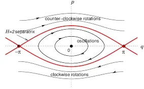
- Can plot momentum and position of a particle.
- Closed loops are called librations
- Unbounded paths are called rotations
- The boundary between the two is called the separatrix
Poisson Brackets
- Suppose that you have some observable $f(q_{i}, p_{i},t)$
- Utilizing the total time derivative and Hamilton’s equations, you show
- $\frac{df}{dt} = [f,H]+ \frac{\partial f}{\partial t}$
- $[A,B] = \frac{\partial A}{\partial q_{i}}\frac{\partial B}{\partial p_{i}}- \frac{\partial A}{\partial p_{i}}\frac{\partial B}{\partial q_{i}}$
- This is the Poisson bracket
- $[A,B] = \frac{\partial A}{\partial q_{i}}\frac{\partial B}{\partial p_{i}}- \frac{\partial A}{\partial p_{i}}\frac{\partial B}{\partial q_{i}}$
- $\frac{df}{dt} = [f,H]+ \frac{\partial f}{\partial t}$
Properties
- $[\alpha f_{1} + \beta f_{2}, g] = [\alpha f_{1}, g] + [ \beta f_{2}, g]$
- $[f,g] = -[g,f]$
- $[f,[g,h]]+[h,[f,g]]+[g,[h,f]] = 0$ (Jacobi identity)
- $[f,gh]= [f,g]h + g[f,h]$ (Leibniz’s rule)
Any object which satisfies the above properties is called a Lie Algebra.
The fundamental Poisson brackets are
- $[q_{i}, q_{j}] = 0 = [p_{i}, p_{j}]$
- $[q_{i}, p_{j}] = \delta_{ij}$
Jacobi Proof Sketch
To prove the Jacobi efficiently, utilize the following notation:
- $[f,g] = \Omega_{ab} \partial_{a} f \partial_{b} g$
- $\Omega_{ab} = \begin{pmatrix} 0 & 1 \\ -1 & 0 \end{pmatrix}$
- $\partial_{a} = \begin{pmatrix} \frac{\partial}{\partial q} \\ \frac{\partial}{\partial p} \end{pmatrix}$ To generalize, you make a block matrix with the on diagonal matrices being $\Omega_{ab}$. YOu also add 2 elements to the partial derivative vector
Hence: $[f,[g,h]] = \Omega_{ab} \partial_{a} f \partial_{b}(\Omega_{cd} \partial_{c} g \partial_{d} h )$ Note down the associated formula for the cyclic permutations, so some index juggling and symmetry abuse, and you can prove it
Poisson’s theorem
- If $\frac{df}{dt} = \frac{dg}{dt} = 0$, then $\frac{d}{dt}[f,g] = 0$
- You can generate a new conserved quantity by taking the Poisson bracket of two conserved quantities
- The new quantity is not necessarily linearly independent from f and g
- You can generate a new conserved quantity by taking the Poisson bracket of two conserved quantities
Canonical Transformations
- We know that the tranformation $Q_{i} = Q_{i}(q,t)$ leaves the form of the Lagrangian unchanged. How does the Hamiltonian change under the same transformation?
- If you let your $P_{i} = \frac{\partial L}{\partial \dot{Q_{i}}}$, then you get the same equations of motion
- What if you start from the Hamiltonian, and make the transformation $Q_{i} = Q_{i}(q_i,p_i,t)$ and $P_{i} = P_{i}(q_i,p_i,t)$. What transformations will preserve the equations of motion?
- The transformations which do preserve the equations are called “canonical”
- A transformation is canonical if the Poisson bracket is invariant w.r.t. changes in coordinates (ie. $[f,g]_{QP} = [f,g]$)
- Assume for now that transformations are time-independent
- This can be proven by observing that $\dot{Q_{i}} = [Q_{i}, H]$
- Expanding the Poisson bracket w.r.t. Q and P, and noting that $\frac{\partial Q_{i}}{\partial P_{j}}$, you recover one of Hamilton’s equations. This can also be done with $P_{i}$ instead
- An equivalent formulation is as follows:
- $[Q_{i}, Q_{j}] = 0$ for all canonical coordinates
- Same for P
- $[Q_{i}, P_{j}] = \delta_{ij}$
- Some examples of canonical transformations:
- $Q_{i} = q_{i}; P_{i} = p_{i};$ is the identity
- $Q_{i} = q_{i}+ \alpha_{i}; P_{i} = p_{i}+ \beta_{i};$ is a translation
- $Q_{i} = p_{i}; P_{i} = -q_{i};$ is like a 90 degree rotation in phase space
- This generalizes to an arbitrary rotation
- This implies that there is no fundamental difference between momenta and coordinates (formally)
- If you write the Lagrangian in terms of the Hamiltonian, then to have a canonical transformation, you must obey $p_{i}\dot{q_{i}}-H = P_{i}\dot{Q_{i}}-K + \frac{dF}{dt}$
- K is some new Hamiltonian, and F is some scalar field which can be added to the Lagrangian to leave it unchanged
- The above can be written as $dF = p_{i} dq_{i} - P_{i} dQ_{i} + (K-H) dt$
- Since there is some interplay between the variables, you can normally reduce F down to a function of two variables
- $q_{i}$ and $Q_{i}$ is type 1
- $q_{i}$ and $P_{i}$ is type 2
- $p_{i}$ and $Q_{i}$ is type 3
- $p_{i}$ and $P_{i}$ is type 4
- To derive the coordinate transform, take the appropriate Legendre transform of F, equate to $dF = p_{i} dq_{i} - P_{i} dQ_{i} + (K-H) dt$, then cancel and match like terms
- F1: $p = \frac{\partial F_{1}}{\partial q}$ and $P = -\frac{\partial F_{1}}{\partial Q}$
- F2: $p = \frac{\partial F_{2}}{\partial q}$ and $Q = \frac{\partial F_{2}}{\partial P}$
- F3: $q = -\frac{\partial F_{3}}{\partial p}$ and $P = -\frac{\partial F_{3}}{\partial Q}$
- F4: $q = -\frac{\partial F_{4}}{\partial p}$ and $Q = \frac{\partial F_{4}}{\partial P}$
- Since there is some interplay between the variables, you can normally reduce F down to a function of two variables
Why We Care
- If you can find the appropriate cannonical transformation, you can directly get the solutions to Hamilton’s Equations without solving them
Liouville’s Theorem
- The Poisson bracket is invariant under a canonical transformations
- The volume in phase space is also conserved under canonical transformations
- Follows directly from taking determinant of Jacobian and utilizing Poisson brackets
- Can also use the fact that $J^{T}\Omega J = \Omega$ where $\Omega = \begin{pmatrix} 0 & I \\ -I & 0 \end{pmatrix}$ is the symplectic matrix. Taking the determinant of both sides yields that $det(J) = 1$, which implies a volume conserving transformation
Canonical Invariants
- Let $Q(t) = q(t+dt) = q(t)+\frac{dq}{dt}dt = q(t)+\dot{q}dt$
- Let $P(t) = p(t+dt) = p(t)+\frac{dp}{dt}dt = p(t)+\dot{p}dt$
- $[Q,P] = [q+\frac{\partial H}{\partial p} dt,p-\frac{\partial H}{\partial q} dt] = 1 + O(dt^{2})$
- Last step is using linearity and utilizing equality of 2nd partial derivatives
- This is called Liouville’s Theorem
Entropy Tangent
- Imagine that you prepare a system at a particular point. There is some uncertainty in the exact location, so draw a disk around it to represent this spread
- As time evolves, you need to evolve the every point in the disk
- Since phase space area is preserved, and each point in the original disk has the potential to move every far apart from each other, we expect the new area to be “wispy” or jellyfish-like
- The phase space area is the same
- The uncertainty in each region remains roughly the same though, so you place the uncertainty circles around each point on the jellyfish
- So, effectively, the area of the uncertainty has increased over time, which is kind of like entropy!
- The above process is called coarse graining. It could be extended to a more realistic Gaussian
Infinitesimal CTs
- Let
- $Q_{i} = q_{i}+ \delta q_{i}$
- $P_{i} = p_{i}+ \delta p_{i}$
- $Y_{i} = y_{i}+ \delta y_{a}$
- $F_{2}(q_{i}, P_{i}) = q_{i}P_{i} + \epsilon G(q,P,t)$
- $\delta p_{i} = -\epsilon \frac{\partial G}{\partial q_{i}}$
- $\delta q_{i} = -\epsilon \frac{\partial G}{\partial p_{i}}$
- $\delta y_{a} = \epsilon [ y_{a}, G]_{y}$
- G is the generating function of the infinitesimal canonical transformation
- As a concrete example, the generator of time translation is the Hamiltonian
- $\delta q_{i} = dt [q_{i}, H] = \dot{q} dt = \delta q_{i}$
Hamiltonian Noether’s Theorem
- Suppose that G generates some ICT
- $Y_{i} = y_{i}+\epsilon [ y_{a}, G]$
- $\frac{dG}{dt} = [G,H] + \frac{\partial G}{\partial t} = \Omega_{ab} \partial_{a}G \partial_{b} H + \frac{\partial G}{\partial t} = \Omega_{ab} \partial_{a} G \partial_{b} y_{c} \frac{\partial H}{\partial y_{c}} + \frac{\partial G}{\partial t}$
- $\frac{dG}{dt} = [G,y_{c}] + \frac{\partial H}{\partial y_{c}} + \frac{\partial G}{\partial t}$
- $\epsilon \frac{dG}{dt} = -\frac{\partial H}{\partial y_{c}} \delta y_{c} + \epsilon \frac{\partial G}{\partial t} = \Delta H$
- So if $\Delta H = 0$, then $\frac{dG}{dt} = 0$
- This is an iff, so you can go the other way
Hamilton Jacobi Equation
- We need to find some canonical transformation that makes $K=0$
- If $K=0$, this implies that the $Q_{i}$ and $P_{i}$ are constants
- Let’s use $F_{2}(q,P,t)$
- $p_{i} = \frac{\partial F_{2}}{\partial q_{i}}$
- $Q_{i} = \frac{\partial F_{2}}{\partial P_{i}}$
- $K = H+ \frac{\partial F_{2}}{\partial t} = 0$
- Hence: $H(q_1,…q_{n}, \frac{\partial F_{2}}{\partial q_{1}},…,\frac{\partial F_{2}}{\partial q_{n}}) + \frac{\partial F_{2}}{\partial t} = 0$
- This is the Hamilton-Jacobi Equation
- We define $F_{2} = S(q_{1},…, q_{n}, \alpha_{1},…\alpha_{n}, t)$
- $\alpha_{i}$ is a set of s constants which we can take to be $P_{i} = \alpha_{i}$
- $Q_{i} = \beta_{i} = \frac{\partial S}{\partial P_{i}} = \frac{\partial S}{\partial \alpha_{i}} (q_{i}, \alpha_{i},t)$
- This can be inverted and solved for the $q_{i}$
- S is given by $S = \int^{t} dt’ L(q(t’), \dot{q(t’)}, t’)$
- You can set the lower bound to whatever you want
- This equation can sometimes be solved via separation of variables
- You make the ansatz $S = \Sigma_{i} W_{i}(q_{i}) + f(t)$
Action Variables
- If we are in a 2s dimensional space, and we have separable system, then we can reduce the problem to motion in s hyperplanes with variables $p_{i} q_{i}$
- Let’s look at a harmonic oscillator
- Let $Q_{i} = \theta$ define an angular which is linear in time
- Let $P_{i} = J_{i}$ is the action variable, which is constant
- You can think of the action variable defining which surface you are on, while the Q defines where you are on the torus
- Hence, we need to find some canonical transformation which has these properties
- $\dot{\theta_{i}} = \frac{\partial K}{\partial J_{i}} = \nu_{i}(J_{i})$
- $\dot{\nu_{i}} = 0$
- $\theta_{i} = \nu t+\beta$
- $\tau_{i} = \frac{2\pi}{\nu_{i}}$
- Need to find $W(q,J) = \Sigma_{i} W_{i}(q,J)$
- $p_{i} = \frac{\partial W}{\partial q_{i}}$
- $q_{i} = \frac{\partial W}{\partial J_{i}}$
- $2\pi = \oint d\theta_{i} = \int \frac{\partial^{2} W_{i}}{\partial J_{i} \partial q_{i}} dq_{i} = \frac{\partial }{\partial J_{i}} \oint p_{i} q_{i}$
- $J_{i} = \frac{1}{2\pi} \oint p(q,J) dq$
- For the harmonic oscillator, can think of this as an area
- $W_{i}(q_{i}) = \int^{q_{i}} p_{i}(\tilde{q_{i}},J) d\tilde{q_{i}}$
- $J_{i} = \frac{1}{2\pi} \oint p(q,J) dq$
Multiperiodic motion
- We know that $\theta_{i} = \theta_{i}+2\pi k$ (ie. is periodic)
- We can then write the y’s (q’s and p’s lumped together in one big 2s vector) as:
- $y = \Sigma_{\vec{k}} A_{k}(J) e^{i(k_{i}\beta_{i})}e^{it(k_{i}\nu_{i})}$
Planetary motion
- $H = \frac{1}{2m}(p_{r}^{2}+\frac{p_{\phi}^{2}}{r^{2}})+V(r)$
- $V = \frac{c}{r}$
- Using Hamilton Jacobi, let $W = W_{r}(r)+\alpha \phi$
- $(\frac{\partial W}{\partial r})^{2} \frac{\alpha^{2}}{r^{2}}+2mV = 2mE$
- $W_{r}(r) = \int ^{r} dl \sqrt{2m(E-V(l))-\frac{\alpha_{\phi}}{l^{2}}}$
- $K = E = \alpha_{1}$ since no explicit time dependency
- $\dot{Q_{1}} = \frac{\partial K}{\partial E} \rightarrow Q_{1} = \beta_{1}+t = \frac{\partial W}{\partial E}$
Liouville’s Integrability Theorem
- If you have a Hamiltonian system with s $q_{i}$ and s independent conserved quantities $\alpha_{i}$ that commute, then the system is integrable
- Independent means that the conserved quantities span a subspace of dimension S
- integrable means that there exist a complete set of action-angle variables
Cannonical Peturbation Theory
- Suppose that you have the Hamiltonian $H = \frac{p^{2}}{2m} + \frac{m\omega_{0}q^{2}}{2}+ \frac{\epsilon m}{4} q^{4}$
- The Hamiltonian has the form $H_{0}+\epsilon \delta H$
- $H_{0}$ has a set of action angle variabled defined for it $(\theta_{0}, J_{0})$
- We want to find a new set of action-angle variables for the peturbed system
- $H(\theta_{0}, J_{0})=H_{0}(\theta_{0}, J_{0})+\delta H(\theta_{0}, J_{0})$
- $H_{0} = H_{0}(J)$ by construction
- The plan: at each new order of epsilon, find a new set of action-angle variables
- The unperturbed variables are given by
- $q = \sqrt{\frac{2J_{0}}{m\omega_{0}}} \sin \theta_{0}$
- $p = \sqrt{2m \omega_{0} J_{0}} \cos \theta_{0}$
- We want to find a generating function $F(\theta_{0}, J_{1})$
- Since this is an infinitesimal transformation, we can write it in the form $F_{2} = \theta_{0}J_{1}+\epsilon G(\theta_{0}, J_{1})$
- You can write all relevant variables in terms of $F_{2}$
- $J_{0} = \frac{\partial F_{2}}{\partial \theta_{0}} = J_{1} + \epsilon\frac{\partial G}{\partial \theta_{0}}$
- $\theta_{0} = \frac{\partial F_{2}}{\partial J_{1}} = \theta_{0} + \epsilon \frac{\partial G}{\partial J_{1}}$
- Since we have no time dependency, we know that K=H
- Making this subtitution into K yields $K_{1} = \omega_{0} J_{1} + \epsilon \omega_{0} \frac{\partial G}{\partial \theta_{0}} + \frac{\epsilon J_{1}^{2}}{m \omega_{0}^{2}} \sin^{4}(\theta)$
- We can utilize a Fourier expansion of G to solve the equation:
- $G(\theta_{0}, J_{1}) = b_{0}(J_{1}) + \Sigma_{n=1}^{\infty} (a_{n}(J_{1})\sin(n\theta_{0})+ b_{n}(J_1)\cos(n\theta_{0}))$
- Alternatively, we can take the angular average, which is
- $<f> = \frac{1}{2\pi}\int_{0}^{2\pi} f d\theta_{0}$
- This yields a more general formula for peturbations: $K = K_{0}(J) + \epsilon <\delta K> = K_{0}(J_{1}) + \epsilon \omega_{0} \frac{\partial G}{\partial \theta_{0}} + \epsilon \delta K$ or $\omega_{0} \frac{\partial G}{\partial \theta_{0}}<\delta K> -\delta K$
- This approach essentially encodes the Fourier trick into it
- We can also encode this in complex numbers:
- $G(\theta_{0}, J_{1}) = \Sigma \tilde{G}(n,J_{1}) e^{in\theta}$
Adiabatic Motion
- Suppose that $H(p,q,\lambda)$ where $\frac{\partial H}{\partial t} \propto \frac{\partial \lambda}{\partial t}$ where $\lambda = \lambda(t)$
- In general, there are no closed orbits and J is not well defined
- If we vary $\lambda$ slowly (or adiabatically)
- $\frac{\frac{d\lambda}{dt} \tau}{\lambda} « \lambda$ where $\tau$ is the period of the system, then you can pretend that there are closed orbits since $\frac{\Delta J}{J} \approx \epsilon^{2}$
- Can show this by expanding the Hamiltonian to first order, using $\cdot{J} = - \epsilon \frac{\partial \delta H}{\partial \theta}$, expanding with Fourier coefficients, then taking the angle average to show $<\cdot<J> = 0$, which implies that it’s order $\epsilon^{2}$
- $\frac{\frac{d\lambda}{dt} \tau}{\lambda} « \lambda$ where $\tau$ is the period of the system, then you can pretend that there are closed orbits since $\frac{\Delta J}{J} \approx \epsilon^{2}$
Quantum
Mach Zender
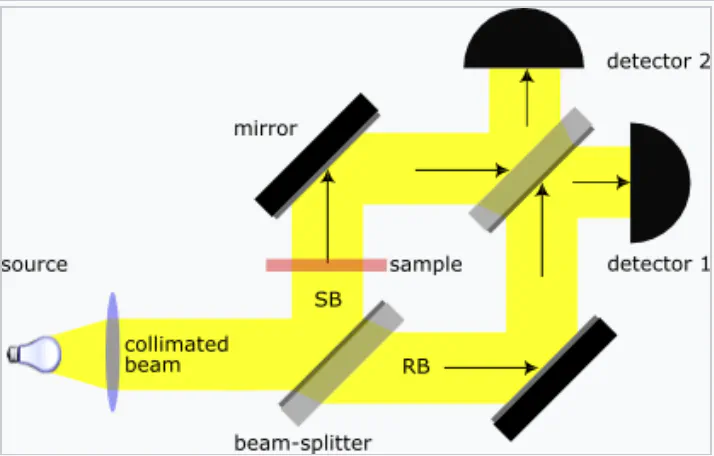
- The above is a Mach-Zender interferometer. If you shine a classical light on the interferometer (and you don’t sample in an arm), you expect to measure all of the light on detector 1
- If you block an arm, you measure 25/25 on each arm
- Say that you reduce the light down to single particles which satistfy $h\nu > E_{work}$. What do you see?
- The probability of the “clicks” follows that of the classical regime (both the blocking and non-blocking case)
- What path does the photon take?
- It doesn’t take a single path, since then you would see 100% in the blocking case
- It doesn’t take both paths, since then you would see clicks in both detectors. But you only see clicks at one detector?
- So… what did it do? It’s hard to describe in English (it’s a superposition of states, which can be described by linear algebra mathematically, but that’s not particularly intuitive…)
- What path does the photon take?
- The probability of the “clicks” follows that of the classical regime (both the blocking and non-blocking case)
Hilbert Space
Linear Algebra Review
- In classical mechanics, we can think of particles as delta functions in phase space: $\rho_{c} = \delta(q-q_{0}, p-p_{0})$
- You can add up points together as long as $a\rho_{c}^{1}+b\rho_{c}^{2} = \rho_{c}^{3}$ where $a+b=1$ and $a,b \geq 0$
- In quantum mechanics, we think of particles as elements in a Hilbert space
- A Hilbert space is a vector space over the complex numbers, with the metric that the inner product between any two elements yields a complex number (denoted as $<x|\Psi> \in \mathbf{C}$)
- We also demand that this inner product is positive definite (ie. the inner product of $<\Psi|\Psi> \geq 0$), with equality iff $|\Psi> = 0$
- Need to complex conjugate the “bra” when doing inner products
- This implies that $<\Psi|x> = <x|\Psi>^{*}$
- A Hilbert space is a vector space over the complex numbers, with the metric that the inner product between any two elements yields a complex number (denoted as $<x|\Psi> \in \mathbf{C}$)
- Physical observables must be Hermetian operators
- This means that $U^{T*} = U$ ( the transpose conjugate is the same as the original matrix)
- This can be denoted by $U^{\dag} = U$
- The analagous real thing of this is a symmetric matrix ($U^{T} = U$)
- It’s also nice if operators are unitary: $U^{\dag} = U^{-1}$
- The analagous real thing of this is an orthogonal matrix
- This means that $U^{T*} = U$ ( the transpose conjugate is the same as the original matrix)
- The trace is defined as $Tr(U) = \Sigma_{i} U_{ii}$
- Fun property of traces: $Tr(ABC) = Tr(CAB) = Tr(BCA)$
- This implies that the trace is invariant under unitary transformations
- $Tr(U) = \Sigma_{i} \lambda_{i}$
- Fun property of traces: $Tr(ABC) = Tr(CAB) = Tr(BCA)$
- The determinant is also invariant under unitary transformations. Also $det(U) = \Pi_{i} \lambda_{i}$
- $det(AB) = det(A)det(B)$
- A unitary matrix has real eigenvalues and it’s eigenvectors forms a complete basis and are orthonormal unless $\lambda_{i} = \lambda_{j}$
- Orthonormal means $<i|j> = \delta_{ij}$
- The outer product is defined as $|y><x|$
- This is a linear operator
- A special outer product is the projection operator: $|\Psi><\Psi| = P$
- $P^{2} = P$
- Eigenvalues must be 1 or 0
Time Evolution
- Suppost that at time $t=t_{0}$, there is some element $|\alpha> = |\alpha, t_{0}>$ such that $|\alpha, t> = U(t,t_{0})|\alpha, t_{0}>$
- where U is the time evolution operator
- We must have that probabilities are normalized
- $<\alpha,t|\alpha,t> = 1$
- We assume that U is the same, regardless of what $\alpha$ you start in
- this implies that $U$ is unitary (ie $U^{\dag} = U^{-1}$)
- The infinitesimal time evolution operator is defined as $U(t_{0}+dt, t_{0}) = I-i\Omega dt$
- Can show that $\Omega$ is unitary via unitary requirement on U
- We make the guess that $\Omega = \frac{H}{\hbar}$, since from classical mechanics, the Hamiltonian is the invariant under time translation
- $U(t+dt,t) = U(t+dt,t)U(t,t_{0}) = (1-\frac{i}{\hbar}H dt)U(t,t_{0}) \rightarrow i\hbar \frac{d}{dt} U(t,t_{0}) = H U(t,t_{0})$
- This is just the Schrodinger equation
- Assuming $\frac{\partial H}{\partial t} = 0$, then $U(t,t_{0}) = exp(\frac{-iH}{\hbar}(t-t_{0}))$
Heisenberg Formulation
- Instead of thinking of the states as a function of time, we can thing of the operators as a function of time
- $A(t) = U^{\dag}(t,t_0)A(t_0)U(t,t_0)$
- This is equivalent to Schrodinger picture since the only observables are expectation values
- Since $|\Psi(x,t)> = U(t)|\Psi(x)>$, we can just think of translating the time dependency from the state to the operator
- The equivalent Schrodinger equation in the Heisenberg picture can be derived as follows
- Take $\frac{d}{dt}(U^{\dag}AU)$, where you keep the central term
- Can take the conjugate of the Schrodinger equation in order to get $\frac{d}{dt}U^\dag$
- Using the fact that the Hamiltonian is Hermetian
- Assume that H commutes with U (ie. that the Hamiltonian commutes with itself at different times)
- Therefore: $\frac{dA}{dt} = \frac{i}{\hbar} [H,A]+\frac{\partial A_{s}}{\partial t}$ where $A_{s}$ is the Schrodinger picture of operator A
- Observe that this is the same as the classical Poisson bracket evolution, but you swap the Poisson bracket with $\frac{-i}{\hbar}$ times the commutator
Compatible Observables
- $[A,B]= AB-BA= 0$ where A and B are operators
- Hence the name commutator: if it’s 0, you can swap around A and B
- If the operators commute, then you can diagonalize each operator in the same basis (not necessarily with the same eigenvalues though…)
- If there are degenerate eigenvalues, then you need to be careful with picking from the degeneracies in the subspace (some type of Gram-Schmidt procedure is necessary)
Symmetries
- Symmetries must be unitary operators to preserve probability
- Discrete Symmetries don’t have to be unitary, since Noether’s theorem doesn’t apply to them
- These are anti-unitary (ie. any transformation with performs the following operation $U(x,y)<x|y> = <y|x>$)
- Discrete Symmetries don’t have to be unitary, since Noether’s theorem doesn’t apply to them
Uncertainty Relationship
- Suppose that $[A,B] = C$
- C is, by construction, anti-Hermetian, which itself is defined as $C = iD$ where D is Hermetian
- $\sigma_{A}^{2} = <A^{2}>-<A>^{2} = <(A-<A>)^{2}>$
- $\sigma_{A}^{2}\sigma_{B}^{2} = |(A-<A>)|\Psi>|^{2}|(B-<B>)|\Psi>|^{2} \geq <\Psi|(A-<A>)(B-<B>)|\Psi>^{2}$
- $\sigma_{A}\sigma_{B} \geq |<\Psi|\frac{1}{2}[\Delta A, \Delta B]+\frac{1}{2}{ \Delta A, \Delta B} |\Psi>| \geq |\frac{1}{2}<\Psi|[\Delta A, \Delta B]|\Psi>|$
- ${A,B}$ is the anticommutator (the curly braces don’t show up well)
- the last inequality comes from the fact that you can drop the anticommutator since it’s purely imaginary
- The $<A>$ is just a number, so it doesn’t affect the commutator, hence $[\Delta A, \Delta B] = [A,B]$
- Hence: $\sigma_{A}\sigma_{B} \geq \frac{1}{2} |<\Psi[A,B]\Psi>|$
- With x and p, we have that $[x,p] = i\hbar$
- $\sigma_{x}\sigma_{p} \geq \frac{\hbar}{2}$
Phase Space Interpretation
- Quantum mechanics doesn’t allow a particle to be at a precise location in phase space
- Particles instead live somewhere inside some disk of whose area is of order $\hbar$
- Can also think of this as quantizing the action variables
Entanglement And Mixed States
- The simplest possible nontrivial QM system is a qubit
- This is a spin $\frac{1}{2}$ particles with eigenbases $|0>$ and $|1>$
- You can think of $|\Psi>$ as living on a Bloch sphere
- Looking at spin along the z-axis, we define the operator
- $\sigma_{z} = \frac{\hbar}{2}\begin{pmatrix} 1 & 0 \\ 0 & -1 \\ \end{pmatrix}$
- Repeated measurements along the same spin axis yields the same spin
- Measurements along different axes randomize the spin
- How do you get a purely unpolarized state?
Mixed States
- We know that $<A> = Tr(A|\Psi><\Psi|)$
- We can represent mixed states via the density matrices:
- $\rho = \Sigma_{i} p_{i} P_{i}$
- $p_{i}$ is the probability that you get the pure state $P_{i}= |\Psi_{i}><\Psi_{i}|$
- A pure state can also be identified by $Tr(\rho) = 1$
- $\rho$ is not a projection operator unless $p_{i}=1$ for only one pure state
- $p_{i}$ is the probability that you get the pure state $P_{i}= |\Psi_{i}><\Psi_{i}|$
- $\rho = \Sigma_{i} p_{i} P_{i}$
- We can then represent expectation values of mixed states as $<A> = Tr(\rho A) = \Sigma p_{i} Tr(P_{i}A)$
- If we have $p_{i}$ be a uniform distribution, we get a true unpolarized state
Von Neumann Entropy
- $\sigma_{V} = -Tr(\rho ln \rho)$
- If you diagonalize $\rho$, then you get $\sigma_{V} = -\Sigma_{i} p_{i} ln p_{i}$
- $\sigma_V = 0$ for a pure state
- $\sigma_{V} = ln(d)$ is the maximum entropy, where d is the dimension of the hilbert space
- The Von Neumann entropy doesn’t change over time
- Let $\rho(t) = U^{\dag} \rho U$
- Taking Von Neumann entropy, and use cyclic property of trace to see the time invariance
Partial Trace (“Tracing Out”)
- Let $|\Psi> \in H = H_{1}\times H_{2}$
- Suppose that we trace out $Tr_{2}(P_{\Psi}) = \Sigma_{i=1}^{d} <i_{2}|P_{\Psi}|i_{2}>$
- ie. You only act on the parts of $\Psi$ which are in $H_{2}$
- Can think of this as a function of how “entangled” the state was
Infinite Spaces
- Suppose that we have a Hermetian operator $X^{\dag} = X$
- We can define $\int |x’><x’| = I$
- We can similarly define expectation values and projections and what not by subbing in summations with integrals
Translation Operator
- $U(\delta t) = exp(\frac{-iH\delta t}{\hbar})$
- $U(dt) = 1-\frac{i}{\hbar}H dt$
- Define $T(\delta x) = T|x’> = |x’+\delta x>$
- $T(dx) = T|x’> 1 - \frac{i}{\hbar} K dx$
- Follows from unitary nature of T
- What is K?
- It’s just p
- Can be shown by acting $x|x+dx’>$, making the T substitution, using the relationship $K = [x,K]+Kx$, simplifying, and then dropping 2nd order terms.
- $T(dx) = T|x’> 1 - \frac{i}{\hbar} K dx$
- Hence, $T(\delta x) = exp(\frac{-ip\delta x}{\hbar})$
- $\Psi(x’) = <x’|\Psi>$
- $\Psi(x’+\delta x) = <x’+\delta x|\Psi>$
- From the above, we can see that $\frac{\partial}{\partial x} \Psi(x’) = <x’|\frac{i}{\hbar}p |\Psi>$
- From the above, we can see that $\frac{\partial}{\partial p} \Psi(p’) = <x’|\frac{-i}{\hbar}x |\Psi>$
- Therefore $x = \frac{-\hbar}{i }\frac{\partial}{\partial p}$ and $p = \frac{\hbar}{i }\frac{\partial}{\partial x}$
- $<x’|p’> = \frac{p’}{p’}<x’|p’>$
- the fraction p’ is just 1. We can pull that inside, then convert the p’ to the operator p: $<x’|p’> =\frac{1}{p’} <x’|p|p’> = \frac{1}{p’} \frac{\hbar}{i}\frac{\partial }{\partial x’} <x’|p’>$
- Solving the above dif. eq yields: $<x’|p’> = N exp(\frac{ip’x’}{\hbar})$
- We know that $<x’|x’’> = |N|^{2}\int exp(\frac{ip’}{\hbar}(x’-x’’)) dp’ = \delta(x’-x’’)$
- This follows by inserting $\int dp’ |p’><p’|$ into the equation
- We define $N = \frac{1}{\sqrt{2\pi \hbar}}$ to allow the above identity
- The above allows use to write:
- $\Psi(x’) = \int dp’ \frac{1}{\sqrt{2\pi \hbar}} e^{\frac{ip’x’}{\hbar}}$
- $\Psi(p’) = \int dx’ \frac{exp(\frac{-ip’x’}{\hbar})}{\sqrt{2\pi \hbar}}$
- These are just Fourier transforms. These conserve probability in each basis
- This allows us to see the Schrodinger equation in two forms:
- The starting equation: $i\hbar \frac{\partial}{\partial t} |\Psi> = H |\Psi>$
- In the position basis with $H = \frac{p^{2}}{2m}+V(x)$, we get the familiar form
- $i\hbar \dot{\Psi(x’)} = \frac{i\hbar^{2}}{2m} \Psi’’+ V\Psi$
Scattering
- You send in some probability distribution onto a potential, and see what fraction gets reflected and transmitted
- Suppose that we have $\Psi(x,t) = A_{+}e^{\frac{i}{\hbar}(kx-Et)}+A_{-}e^{\frac{i}{\hbar}(-kx-Et)}$
- We can construct any function out of some combination of left and right moving waves (Fourier decomposition)
- We can imagine these waves coming from the left and the right (+ from the left (right moving wave) and - from the right (left moving wave))
- Typically, $B_{-}$ (the incident wave from the right)
- We can couple the incident waves to the outgoing waves via the S matrix
- $\begin{pmatrix} S_{11} && S_{12}\\ S_{12} && S_{22}\\ \end{pmatrix} \begin{pmatrix} A_{+} \\ B_{-}\end{pmatrix} = \begin{pmatrix} A_{-} \\ B_{+}\end{pmatrix}$
- S is a unitary matrix (can see from probability conservation considerations)
- After matching the 0th and first derivatives at the boundaries, you can determine the coefficients and calculate
- $R = |\frac{A-}{A+}|^{2}$
- $T = |\frac{B-}{B+}|^{2}$
Probability Current
- If we take the $\frac{d}{dt}|\Psi|^{2} = \frac{d}{dt} \rho$, apply Schrodinger’s equation on the time derivatives, cancel some terms, we can see that
- $\frac{\partial}{\partial} \rho = \frac{\partial}{\partial x} j$
- $j = \frac{i\hbar}{2m}(\Psi^{*}’\Psi-\Psi^{*}\Psi’)$
- The obvious extension is $\frac{\partial}{\partial t} \rho -\nabla \cdot \vec{j} = 0$
- This is just the conservation of probability
- $\frac{\partial}{\partial} \rho = \frac{\partial}{\partial x} j$
Delta Function
- Takes the form $V(x) = \alpha \delta(x)$
- The 0th derivative condition is trivial ($A_{+}+A_{-} = B_{+}$)
- The first derivative is non-trivial. If you integrate the schrodinger equation around x=0 (ie. the spike of the delta), you can take the limit as $\epsilon=0$, you can get a condition which relates the derivative on the left to the derivative on the right
- Solving that linear system leads to
- $R = \frac{\beta^{2}}{1+\beta^{2}}$
- $T = \frac{1}{1+\beta^{2}}$
- $\beta = \frac{m^{2}\alpha^{2}}{k^{2}\hbar^{2}}$
Path Integral
- Imagine a wavefunction in the position basis: $\Psi(x,t) = <x|U(t)|\Psi> = \int dx’ G(x,t,x’,t_{0}) \Psi(x’,t_{0})$
- Can think of G as the green’s function/propagator/impulse response (ie. the systems response to a delta input function)
- This is just $G(x,t,x’,t_{0}) = <x|U(t,t_{0})|x’>$ (insert $|x’><x’|$ into $\Psi$ definition)
Free Particle
- $H = \frac{p^{2}}{2m}$ and $U(t,t_{0}) = exp(\frac{-ip^{2}(t-t_{0})}{2m\hbar})$
- $G = <x|U(t,t_{0})|x’> = \int <x|U(t,t_{0})|p’><p’|x’>$
- Recall $\frac{e^{\frac{ipx}{\hbar}}}{\sqrt{2\pi \hbar}}$
- It can be shown that $G = \sqrt{\frac{m}{2\pi \hbar (t-t_{0})}} exp(\frac{im(x-x’)^{2}}{2\hbar(t-t_{0})})$
- Recall for a classical free particle: $L = \frac{m\dot{x}^{2}}{2}$. The action S is $S = \int dt L = \frac{m}{2}\frac{(x-x’)^{2}}{t-t_{0}}$
- We see that $G = exp(\frac{i S}{\hbar}) \sqrt{\frac{m}{2\pi \hbar (t-t_{0})}}$
- The prefactor is related to the second derivative of the action
Saddle Point Approximation
- let $N = \int_{-\infty}^{\infty} dx e^{-Nf(x)} \approx e^{\N f(x_{s})} \sqrt{\frac{2\pi}{N f’’(x_{s})}}$
- $x_{s}$ is the saddle point
- In quantum mechanics, we can think of N as $\frac{i}{\hbar}$ and $x_{s}$ as being the classical action along the classical path
Path Integral Proof
- Let $U(t_{N},t_{0}) = \Pi_{i=1}^{N} U(t_{i}, t_{i-1}) $
- $G(x,t,x_{0},t_{0}) = <x|U(t,t_{0})|x> = <x|U(t,t_{N})U(t_{N},t_{N-1})…U(t_{1},t_{0})|x>$
- We can insert a complete set of states $\int dx_{i} |x_{i}><x_{i}|$ for each intermediate U. We see that each U turns into a Greens function which propagates the state a little bit
- $G(x,t,x_{0},t_{0}) = \int dx_{i} \int dx_{2}… \int dx_{N} G(x,t,x_{N},t_{N})G(x,t,x_{N-1},t_{N-1})…G(x,t,x_{0},t_{0})$
- $G(x,t,x’ t_{j-1}) = <x|U(t_{j},t_{j-1})|x’> = <x|1-\frac{iH\delta t}{\hbar}|x’> = <x|exp(\frac{iT\delta t}{\hbar})exp(\frac{iV(x)\delta t}{\hbar})|x’>$
- Can pull out the potential term by acting it on the $|x’>$ eigenstate, converting x to x'
- Can convert remaining T component via $<x|exp(\frac{-iT(p)\delta t}{\hbar})|x’> = \sqrt{\frac{m}{2\pi i \hbar \delta t}} exp(\frac{im(x-x’)^{2}\delta t}{2\hbar \delta t^{2}})$
- Can take limit as N aoes to infinity to get that $G(x,t,x_{0}, t_{0}) = \int_{x_{0}}^{x(t)} [dx(t)] exp(\frac{i}{\hbar} S[x(t)])$
- $[dx(t)] = \lim_{N\rightarrow \infty} \int \Pi_{j=1}^{N}(dx_{j}\sqrt{\frac{m}{2i\pi \hbar (\frac{t-t_{0}}{N})}})$
WKB
- We can write the wavefunction as $\Psi(x,t) = \sqrt{\rho(x,t)}exp(\frac{iS(x,t)}{\hbar})$
- $\rho \geq 0$
- $S^{*} = S$
- S, at this state, doesn’t have a physical meaning
- This comes from the fact that any complex number can be represented as $z = |z|exp(i\phi)$
- Plugging in this definition into the probability current definition yields that $\frac{\rho \nabla S}{m} = \vec{j}$
- Plugging in this definition of the wavefunction to the Schrondinger equation, and then only keep terms of order $\hbar^{0}$ yields that $\frac{1}{2m}|\nabla S|^{2}+V(x)+ \frac{\partial S}{\partial t} = 0$
- We can think of this as the limit where $\hbar |\nabla^{2} S| « |\nabla S|^{2}$, which is roughly the same as saying $\frac{S}{\hbar} » 1$
- Alternatively, imagine a constant potential. $\nabla^{2}S$ is identically 0. For small spatial variations, we expect the deviation from the constant potential to be small. Hence the above approximation is reasonable
- This is just the Hamilton-Jacobi equation, so we can think of S as being the action!
- We can separate the action like $S(x,t) = W(x) - Et$, just like classical mechanics. Plugging in this ansatz to the Hamilton Jacobi equation (in 1D for simplicity) yields
- $i\hbar\frac{\partial^{2} W}{\partial x^{2}}- (\frac{\partial W}{\partial x}) ^{2}+K^{2}(x) = 0$
- We let $W = W_{0}+W_{1}$, where $W_{0}$ is of order 0, and $W_{1}$ is of order one. We only keep terms of order one in the approximation
- $K(x) = \sqrt{2m(E-V(x))}$
- Neglecting the $\hbar$ term yields that $W_{0}’ = \pm i K(x)$
- $W_{0} = \pm \int K(x’) dx'$
- To get the density, we need a higher order approximation. We get this by plugging in $W_{0}$ to the original equation: $\frac{\partial W_{1}}{\partial x}^{2} = K^{2} + i\ddot{\hbar W_{0}}$
- Solving this dif. eq for W yields $W \approx W_{1}(x) = \pm (\int dx’ K(x’)) + \frac{i}{2} \hbar ln K(x)$
- This implies that $\Psi_{E}(x,t) = \frac{1}{\sqrt{K(x)}} exp(\frac{\pm i}{\hbar} \int K(x’)dx’)$
- This is the WKB approximation!
- $i\hbar\frac{\partial^{2} W}{\partial x^{2}}- (\frac{\partial W}{\partial x}) ^{2}+K^{2}(x) = 0$
- What can the WKB do?
- It’s crap at approximating the ground state (which makes sense)
- It’s pretty good for higher order eigenstates
- It’s pretty good for scattering problems (You can approximate how the wavefunction changes as it passes through a janky potential), which means you can a good grasp on what T and R are